Demonstration Movies
Computer Generated Atoms and Molecules
Units of Measurement in the Computer-Generated world
Dynamics in the Computer-Generated World
Energy and Temperature in the Computer-Generated World
Chemistry of the Computer-Generated World
The Universal Application is a model of nanoscale world. We suggest that you explore it! To do so, you can either watch the movies that we have prepared for you or create new ones of your own. The world that we are suggesting you to explore consists of rather simple atoms, much like Democritus of ancient Greece could have imagined. If we define species of those atoms along with a few parameters to describe their properties, the system can mimic a variety of phenomena of the real microscopic world.
We suggest that you first watch our movies: This does not take any effort. If you like them, you can try to be creative. This may take some patience and effort, but does not require knowledge beyond what most college freshman have.
This material is organized as follows. We first describe our simplest movies. Then we go a little deeper and explain how our model world works: what atoms look like, how they combine into molecules, and how they interact and move. After that, we specify in more detail how the properties of a particular system of atoms are encoded for the program to work. Finally, we give more specific suggestions for creating a good movie
Our first movie is called StatesofMatter. It shows an ordinary simple
system of identical molecules. What you see here is the chaotic motion of all
the molecules. This is called thermal motion, or, if you prefer, Brownian motion.
Note that in this first movie all of the molecules are of the same kind; they make up a pure substance, like pure water. Molecules never penetrate each other, meaning that there are forces that repel molecules from each other when they come close (which, of course, happens from time to time). In this sense, the gas is not ideal. One can ``measure'' its pressure and see that it deviates from Boyle's law. At the same time, it is hard to tell if there are any forces of attraction. But if you look carefully, you can see a slight manifestation of the attractive forces: When two molecules happen to be relatively slow (some of them are always slower than others) and two slow ones meet, they remain coupled for quite some time. This suggests that something interesting can happen at lower temperatures, where all of the molecules move more slowly.
Watch the temperature graph, at certain moment of time we will reduce the temperature, which in our simulation is proportional to the average kinetic energy of the molecules.
The second part of our movie is just a little bit more complex than first one. The molecules are the same as in the first part, except now the temperature is lower. What happens to familiar liquids when you heat them up? What happens to water in your coffeemaker or kettle when you are preparing your breakfast? Yes, of course: it boils and vapor comes off. Accordingly, if you take a vapor and cool it down, you expect to see condensation. You can see in this movie how this looks at the level of molecules.
When the temperature goes below the freezing point, the little crystals start to grow out of the liquid. You can see this process in the third part of the movie, called ``Crystallization.''
Thus, forces of attraction are directly responsible for phase transitions, such as condensation and crystallization. However, this was a pure substance. What can happen if we mix two different substances?
``Phase Segregation'' is our second movie, and it is again about a simple
nonpolymeric liquid. This time we show what happens if we try to mix two liquids,
such as water and oil, that tend not to mix. You can see that the different
types of molecule do indeed get segregated. Not perfectly, because there is
some diffusion of one component into the other, but most of the molecules segregate
very well.
How did we do that? We took two types of molecules very similar in size that interact in a peculiar way: Similar molecules attract each other, different ones repel each other. Not surprisingly, they don't tend to mix.
We hope that these examples are sufficient to give you an idea of the richness of our nanoscale world.
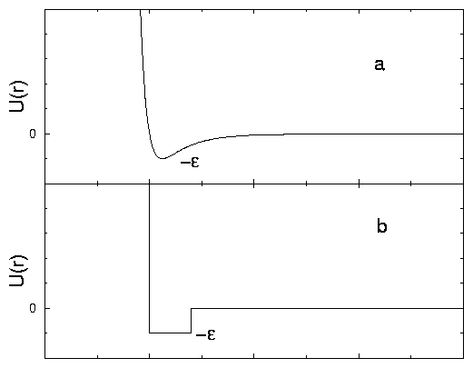
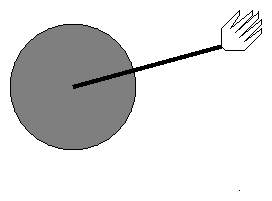
The atoms of the computer generated world are much more simplified that in reality. They are much like billiard balls, but not exactly. The atom shown in Figure 1.3 has a hard core shown dark in the figure, which is indeed exactly like a billiard ball. It is this core that is shown in the movies. Other atoms can never penetrate there. The lighter area around the core in Figure 1.3 means the region where other atoms feel attracted to this atom, if they come this close. Remember that normally there are interactions between atoms, molecules and other particles in the real world. In Figure 1.2, we show the real-world potential in comparison with the interaction potential used in our simple model.
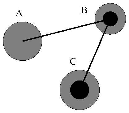
Finally, each atom can have several ``arms,'' which serves to combine atoms into molecules. Each arm can hold one (and only one) partner. For example, if the arm of atom A holds B, the arm of B holds C we get a three-atom molecule whose ``chemical formula'' looks like ABC. This is shown schematically in Figure 1.3.
Thus, to model molecules we must specify from the very beginning the entire list of connections. That is, for each atom, we have to specify which partner will be connected to this atom's arms.
What do the model atoms and model molecules stay for? What do we try to model and present with them? Certainly, model atoms are NOT necessarily pretend to model real atoms. They may as well represent much larger ``clumps'' of material. For instance, when we model polymer chains, we represent each monomer as one model atom. Clearly, in this case each model atom plays the role of a pretty big molecule. As a matter of fact, however, they may represent even bigger particles, such as seeds of dust or even viruses: this large particles, when suspended in liquid, can undergo various transformations which can well be modeled using our model interaction. Thus, we speak about atoms and molecules, but the user of our program must keep in mind that they can mimic a lot of various situations of the real world.
As our model atoms may represent a variety of different real systems, the absolute values of the sizes and mass lack any meaning. Similarly, absolute values of any time intervals are also meaningless. The only relevant figures stay for ratios of different length mass and time scales.
Usually, in our computer-generated world we assign each `atom' to have mass a unit mass, a diameter of 10 units and the interaction is 1. In order to translate these units into the units of the real world we must know which substance we simulate. We know that the mass of an argon atom is 6.634·10-26 Kg. and his diameter is 34.9 A0 and the energy of interaction between atoms of argon is 1.654 ·10-21 J. In the simulation file format there is a line, called Real Units. In that line we must enter numbers for the length, mass and energy. Then, the program will automatically convert all the quantities of interest into scientific units: meters (length), kilograms (mass), seconds (time), joules energy), Pascal (pressure) and kelvin (temperature).
Geometry of the computer world cannot model an infinite system. So in all our movies and simulation the system has a finite size. The Universe, in our computer simulations is a three-dimensional or two-dimensional box with fixed x, y and z dimensions. Sometimes, when the specific effect can be absorbed in two-dimensional simulations, we use two-dimensional simulations, which are much easier for visualization. The speed of computer simulations depends on the number of atoms involved. In really experiments a laboratory sample has about 1023 molecules. In computer generated world, we cannot simulate, at present, much more than 10000 particles, even on a very fast computers. In order to overcome this difficulty, we introduce very peculiar properties on the boundaries of our computer generated Universe. Indeed, what happens when, say, a model atom approaches lower boundary of the box? The geometry of the model world is defined in terms of the so-called periodic boundary conditions: this means that the atom approaching a boundary does not ``see'' anything special, but goes directly to the opposite boundary. Watching movies, you will see numerous examples when atoms seem to disappear behind the frame. Don't worry, they will not be lost: if the atom goes down to the lower boundary, it appears immediately from the upper one; if it seems to disappear to the right, it appears immediately from the left, etc.
How do atoms move in the model world?
They obey standard laws of classical mechanics, Newton's laws. As long as an
atom is far enough from all others, no forces act on it, and inertia makes it
move straight with constant velocity. Of course, velocities of atoms change
upon their collisions: when two atoms come close enough such that each enters
the region of attraction surrounding the other (see Figure 1.2),
then both of them get faster according to energy and momentum conservation.
To be a little more specific, imagine that atoms A and B are colliding. The
time of collision and the coordinates of atom centers can be determined from
their present coordinates and velocities. This is a standard problem of analytical
geometry in which the time of the collision is given by a root of a quadratic
equation. This pair is characterized with the interaction range RAB
and interaction strength (or potential energy) eAB. Imagine now the
line that connects centers of the two model atoms precisely at the moment when
they first touch (i.e., when their centers are precisely RAB apart).
At this moment, for each of the atoms two components of the velocity vector
that are perpendicular to the center-to-center line remain unchanged. As to
the velocities components along this line, they change according to the following
simple equations:
|
||||||||||||||||||||||||
Clearly, when two atoms come even closer, their centers approach the distance rAB and touch each other's hard core they get reflected perfectly, just like billiard balls. Again, two components of velocities that are perpendicular to center-to-center line remain unchanged, while components along this line change again according to conservation laws (1.1), except this time there is no potential energy e involved. In this case the Eq. (1.1) has one obvious solution: vA = vA¢, vB = vB¢. This corresponds to the unphysical situation in which atoms continue to move through each other. However, quadratic equation always has the second solution which corresponds to reflection. In the simplest case of equal masses (mA = mB) this second solution is especially simple - atoms simply exchange their velocities: vA¢ = vB, vB¢ = vA.
Similarly, when two atoms are close enough and are within each other's attracting (or repelling) region, but are going to leave that, they get slower (or faster). Of course, they obey again the same conservation laws, except this time potential energy e plays the opposite role (or enters the other side of equation), because particles have potential energy eAB before and don't have it after. If the equation Eq. (1.1) does not have real roots - as it often happens with quadratic equations - then the atoms do not exit the potential well, but just undergo the ``internal reflection.''
Finally, similar rules apply for any two atoms that are connected by an arm. Arm acts actually as an infinitely high potential barrier that does not allow two connected atoms to farther apart than the arm's length DAB. More specifically, as long as two connected atoms A and B are closer than DAB, they do not exert any force on each other; as soon as they approach the distance DAB, they undergo ``internal reflection,'' that is, their velocities transform according to the same conservation principles (1.1) (without any potential energy e involved). There is also minimal distance dAB for connected atoms, and they undergo elastic reflection if they come closer then dAB. In most cases, dAB = rAB, but the program allows these two parameters to be different.
In the computer generated Universe, although the interactions rules are much simpler than in reality, where the interactions between atoms obey laws of quantum mechanics, we find that this model can account for almost all the phenomena that exist in the real nanoscale world except some phase transitions that occur at extremely low temperatures, such as recently observed Bose-Einstein condensation. Thus, to know everything about how all atoms move in the system computer has to solve a couple of simple quadratic equations (1.1) every time two atoms come close to each other. In fact, it has to solve it many-many times, but still the equations are fairly simple. This is why even modest computer power is sufficient to follow interesting effects in the computer generated world.
In the computer generated world, just as in the real one, energy of any closed system is conserved. In particular, total energy of the entire Universe, i.e., of the entire box with atoms and molecules, is conserved - unless we choose to change energy by heating it or cooling it down. This simulation corresponds to the laboratory experiments in which the system is thermally isolated.
We used to describe various objects
of the real word in terms of temperature, and temperature is related to the
average kinetic energy of the chaotic thermal motion:
|
(1.2) |
In our computer-generated world,
we measure temperature in the same units as energy and thus we have kB
= 1. If we specify for our simulation real units, we measure temperature in
Kelvins and use the standard value of kB. In many laboratory experiments,
the total energy of the system is not conserved. Instead the system is either
in thermal exchange with the heath bath at certain temperature. By example,
it is heated up by the stove or is cooled down by the refrigerator. If we want
to simulate such experimental conditions, we measure the temperature T of our
simulated system according to equation 1.2 at certain moment
of time. If T = T0, we do nothing, if T ¹ T0 then we change
the temperature of the system. The new temperature is defined to be
|
(1.3) |
During the first part of the movie the temperature of the thermal bath was T0 = 2, during the second part the temperature was T0 = 0.6 and during the third part T0 = 0.3. The heat exchange coefficient a = 0.01.
In our computer-generated universe particles may represent single atoms, molecules or even larger scales objects like viruses, pollen or dust particles. Each particle in our simulation is characterized by its type , which is represented by different color on the screen. All particles of the same type has the same diameter and mass. The interaction parameter rAB, RAB, eAB, dAB and DAB between two particles depend only on their types A and B. The most simply way of thinking about the types of particles is to assume that the type represent a chemical element. In some movies, we directly name the types of particles as `Oxygen', `Hydrogen', 'Argon', etc..In order to make our computer universe closer to reality we introduce chemical reactions between particles of different types. In general, particles of type A and B may react when they arrive at distance RAB and change their type to C and D, specified by different interaction parameters. After the reaction, the particles may form a chemical bond specified by the distances DCD and dCD. The details of how to model reactions are presented in Section. 2.7
From the discussion above, we are ready to specify all parameters that must be known about the system of model atoms. We have to make a clear distinction between ``physical'' parameters that control the motion of model atoms and other parameters that define the way the system appears on the screen. Let us begin with physics. To specify the system, we need to know:
To specify the screen appearance of the system, we need to know the radius rA for each atom type and also its color.
NOTE: rAB here is the minimal distance between the centers of the particles of types A and B. If the distance between the centers of particles is less than RAB, the particles interact with energy eAB, otherwise the particles do not interact. Obviously RAB should be always larger than rAB. In almost all our simulations rAB = dAB = rA+rB, where rA and rB are the radio of the corresponding images that appear on the screen. This convention ensures that in the two dimensional case the atoms move on the screen like billiard balls: at the moment of their collision their visible hard cores touch each other but never intersect. However there is a possibility to define rAB and dAB independently of rA and rB.
When you watch the movies featuring the ``events'' in our computer-generated universe, you may ask yourself: what is so specific about these movies? Are they any better than many other computer generated movies with a variety of characters and breath breaking stories? Unlike other movies, however, we do not control our characters, they do whatever they do according to their own rules, and actually very simple ones: all they know is conservation principles (1.1), and nothing else. And yet, despite this primitive and unanimated character of the laws governing our universe, the universe itself appears to be unbelievably rich. It is almost like a difference between a child who speaks him/herself, albeit with a primitive vocabulary, and a puppet that speaks perfectly, but with an actor behind the scene. Our computed-generated universe is truly amazing precisely because there is nobody behind!