Virtual Molecular Dynamics Laboratory:
Bridging the Gap Between the Microscopic and Macroscopic
Center for Polymer Studies
Science and Mathematics Education Center
Boston University
This material is based upon work supported by the
National Science Foundation under Grant Nos. MDR-9150079,
CDA-9616565, and ESI-9553883. Any opinions, findings, and
conclusions or recommendations expressed in this material are
those of the author(s) and do not necessarily reflect the views of
the National Science Foundation.
Virtual Molecular Dynamics Laboratory:
Bridging the Gap Between the Microscopic and Macroscopic
|
The text includes an accompanying CD-ROM of software
(we call SimuLabs) for Windows platform. Macintosh, Unix,
and Spanish
versions are available via our Web site:
|
http://polymer.bu.edu/vmdl |
Comments and feedback are most appreciated and can be sent by email to:
|
|
|
Contents
Overview
Simple Molecular Dynamics Feature Tour
1 Temperature and States of Matter
1.1 States of Matter
SL 1: Temperature and the State of Matter
1.2 Temperature
HO 1: Observing Particle Motion in Hot and Cold Water
SL 3: Velocity Distribution
1.3 Research Projects
Research Project 1: States of Matter
Research Project 3: Velocity Distribution
Research Project 5: Velocity Distribution II
Research Project 7: Velocity Distribution III
Research Project 9: Velocity Distribution IV
2 Ideal Gases
2.1 The Concept of Pressure
HO 3: Tire Pump and Coil Spring
HO 5: Atmospheric Pressure
2.2 Boyle's Law
SL 5: Qualitative Investigation of Boyle's Law
SL 7: Quantitative Investigation of Boyle's Law
2.3 Temperature
HO 7: The Subjective Sensation of Temperature
HO 9: HandsOn: Galileo's Thermometer
SL 9: Galileo's Thermometer - Movie
2.4 Charles Law
SL 11: Charles' Law - Movie
2.5 Gay-Lussac Law
SL 13: Gay-Lussac Law
2.6 Avogadro's Law
SL 15: Avogadro's Principle
SL 17: Avogadro's Principle Movie
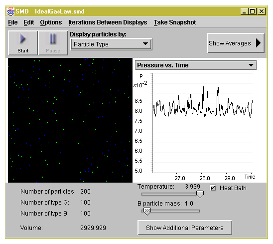
2.7 Ideal Gas Law
SL 19: Ideal Gas Law
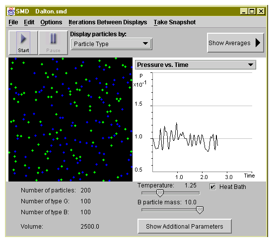
2.8 Dalton's Law
SL 21: Dalton's Law
2.9 Research Projects
Research Project 11: Boyle's Law
Research Project 13: Gay-Lussac Law
Research Project 15: Charles' Law
Research Project 17: Avogadro's Principle
Research Project 19: Ideal Gas Law
Research Project 21: Gay-Lussac Law II
3 Energy and Intermolecular Forces
3.1 Intermolecular Forces
SL 23: Intermolecular Forces
3.2 Kinetic and Potential Energy of Particles
SL 25: Kinetic and Potential Energies of Particles in Gas State
SL 27: Kinetic and Potential Energies of Particles in Liquid State
SL 29: Sublimation, Deposition, and Triple Point.
A Answer Key
B Simple Molecular Dynamics: A Quick Reference
C Outline of Entire Virtual Molecular Dynamics
Overview
| Principal Research Scientist: | Sergey Buldyrev |
| Project Director: | Paul Trunfio |
| Teacher Developers: | Reen Gibb |
| Joseph Jordan |
| Research Scientists: | Lidia Braunstein |
| Sergei Siparov |
| Programmers: | Amit Bansil |
| Anna Umansky |
| Web Developers: | Tim Blount |
| Assessment Coordinator: | Mary Shann |
| Principal Investigator: | H. Eugene Stanley
|
Our classroom experience and research have revealed a startling
discrepancy between the mental models of microscopic processes
possessed by students and those possessed by research scientists.
In many courses, students are asked to learn about and believe in
a macroscopic world without any direct information on which to
base the belief. Research scientists, on the other hand, have a
mental model in which macroscopic events are understood in terms
of the microscopic behavior of a huge number of individual
particles.
Our VIRTUAL MOLECULAR DYNAMICS LABORATORY addresses this problem by
providing a set of research-based molecular dynamics software tools and
project-based curriculum guides. The VIRTUAL LABORATORY enables the
student to visualize atomic and molecular motion, manipulate atomic
interactions, and quantitatively investigate the resulting macroscopic
properties of a range of biological, chemical, and physical systems.
For example, our software package SIMPLE MOLECULAR DYNAMICS (SMD)
allows students to manipulate parameters such as pressure, volume,
temperature, particle number density, and particle mass. Students
are also able to design their own experiments, visualize atoms and
their behaviors, and obtain in-depth, quantitative data which they
can graph in many different ways. For example, students can copy
and tile graphs and discover how various parameters such as
potential energy, kinetic energy and total energy versus time
relate to one another. Investigations include topics such as:
states of matter, enthalpy, Boyle's Law, Charles' Law, Ideal Gas
equation, Gay-Lussac's Law, Avogadro's Principle, Dalton's Law,
diffusion, Graham's Law, kinetic molecular theory, and Maxwell
distribution of velocities. The accompanying SIMPLE MOLECULAR
DYNAMICS PLAYER (SMDPlayer) allows students to view and analyze
movies they have created themselves of previously-saved
simulations.
Accompanying curriculum guides are a collection of project-based
" hands-on'' and " simulab'' activities that are meant to enhance
existing curricula. The " hands-on'' activities hook the students'
interest and focus their attention on the macroscopic phenomena. Then
they investigate the underlying atomic dynamics using the " simulab''.
Each simulab consists of a brief discussion of the concept to be
investigated, learning goals, procedure, questions integrated
throughout, and a teacher's guide.
Other applications currently under development include UNIVERSAL
MOLECULAR DYNAMICS which allows students to design simulations of
simple chemical reactions, build complex chemical compounds such
as polymers, and model complex systems such as diffusion chambers,
cell membranes, or internal combustion engines. Also under
development is the three-dimensional water application, which
introduces students to the microscopic dynamics of water by
simulating how water properties arise from hydrogen bonds and from
the geometry of bonding interactions and the dynamics of the
solvation process.
We have recently been awarded a grant from NSF for
a series of nationwide teacher training workshops using the VIRTUAL
LABORATORY. Beginning in 2001, our workshops will
feature annually two 2-week
summer institutes,
three 3-day regional workshops, and science convention workshops
The project's major features are to (1) prepare 336 high
school chemistry, biology, and physics teachers to incorporate the
VIRTUAL LABORATORY curriculum
into their introductory science classrooms, (2) introduce these
teachers to the role of mentoring in a cooperative learning classroom
environment in which students act as research workers, learning through
hands-on activities, laboratory experiments, and visual and interactive
computer models of chemical, physical, and biological systems, (3)
encourage participating teachers to develop new activities, approaches
and lessons utilizing the computer as a simulator, and (4) develop
online teacher resources including lesson plans, assessments.
Simple Molecular Dynamics Feature Tour
Chapter 1
Temperature and States of Matter
Sensations of temperature are a part of everyday
experiences. My friend's hand is warm. The ice in my drink is
cold. Florida in July is hot. When we quantify these sensations
by measuring temperature, we usually find: the warmer the
sensation the higher the temperature.
We also know from experience that temperature can affect the `state' of
matter. Water becomes ice when we put it in the freezer and steam when
we boil it on the stove.
The first step towards uncovering the mystery of temperature was
made more than two thousand years ago when the ancient Greek
philosopher Democritus formulated the hypothesis that all
objects are made of invisibly small, constantly moving particles
called atoms. It was not until the mid-nineteenth century, that
scientists built upon the ancient atomic hypothesis to
formulate a model of what the individual atoms or molecules might
be doing that could explain temperature and the state of matter.
1.1 States of Matter
|
|
Discuss the following questions:
Q1.1: What are the
states of matter?
Q1.2: How are ice,
liquid water, and steam similar?
Q1.3: How are ice,
liquid water, and steam different?
Q1.4: Imagine that
you could make a " microscopic'' dive into a pool of water and see
the individual water molecules. What do you see happening to the
molecules as the water is cooled and ice begins to form?
Q1.5: What would you
see as water is heated and begins to vaporize?
|
|
|
| |
BEGIN ACTIVITY
SimuLab
1: Temperature and the State of Matter
|
|
Your objective is to:
Recognize the differences between solid, liquid, and gas from the
microscopic point of view.
You will be able to:
Describe the phase transition from liquid to solid and from liquid to
gas in molecular terms.
Contrast the motion of particles in the solid, liquid and gaseous phase.
Describe a liquid-gas equilibrium.
Describe the relationship between states of matter and
temperature.
|
|
|
| |
|
|
Q1.6: Describe, in drawings and in words, your conception of the
molecular structure of a substance in the solid, liquid, and gas
states.
|
|
|
| |
|
|
Q1.7: Describe what happens when we heat a solid in terms of particle
motions and overall structure?
|
|
|
| |
| |
1. Open SMDPlayer, select
IntroStatesofMatter from the StatesofMatter
folder. Press Play. Study the captions and follow the
instructions. When you are finished, select File - Quit
|
| |
| |
This is an introductory movie that visualizes
the three states of matter at the molecular level and the effect of
increasing temperature.
|
| |
|
|
Q1.8: In the introductory movie we saw that as we increase the
temperature, solid melts into liquid and liquid evaporates into
gas. Describe, in drawings and in words, what would happen as we
decrease the temperature of a gas? (Answer such questions as: Do
the molecules move faster or slower? Does the gas expand or
condense?)
|
|
|
| |
| |
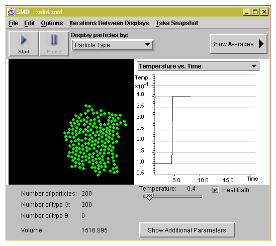
2. Open SMD, select Solid in the
States of Matter folder. Press Start. In order to
speed the simulation switch Iterations Between Displays to
100.
|
| |
| |
In this experiment you are
visualizing 200 particles at the molecular level. The particles
are in the solid state at temperature T=0.1 as shown in Figure
1.1. Our program uses computer units for all the
parameters. You can see temperature and all the other parameters
in real units by selecting Show Averages and then selecting
Show Real Units.
|
| |
Figure 1.1: You see 200 particles at a temperature far below the
freezing point of the substance we are simulating. The horizontal
axis of the graph shows the simulation time. The vertical axis
shows the temperature of the system. The particles are frozen in a
triangular crystal.
| |
3. Select Display Particles by:
Trajectories. Wait no more than 10 time units. Pause the
simulation. Select Take a Snapshot - Screen. When the
dialog box with the Title of the Picture appears type in: " Solid
(T=0.1)'' and press Ok.
|
| |
| |
You are saving
a snapshot of the trajectories of particles in the solid state for later
comparison. Trajectory is another word for the path a particle travels
over time.
|
| |
|
|
Q1.9: Which phrase best describes the trajectories of particles. " The
particles appear to be . . .''
(a) fixed in position
(b) slightly wobbling around a fixed position
(c) moving along in curved lines
(d) moving along straight lines
|
|
|
| |
| |
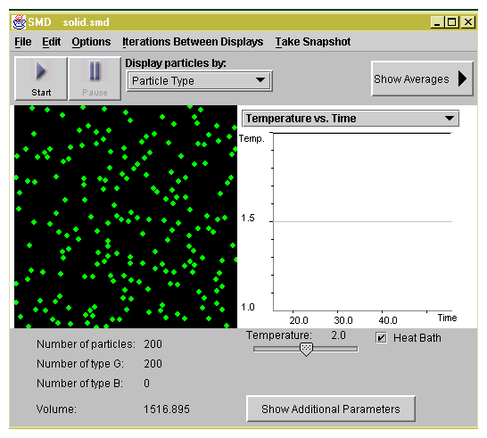
4. Select Display Particles by: Particle
Type. Using the scroll-bar increase the Temperature to T = 0.4. Press Start. Wait at least 20 time units for the
particles to spread.
|
| |
| |
As the temperature
increases, the regular pattern of the solid is destroyed as shown
in Figure 1.2. The molecules begin to move more
freely.
|
| |
Figure 1.2: Your system undergoes a phase transition from the solid
state to the liquid state. The graph shows the change in the temperature
that you made in Step 4.
|
|
Q1.10: Predict what would happen if you lower the temperature back
to T = 0.1. Time permitting, check you prediction. Make sure you
then set the temperature back to T = 0.4 and wait again for 20
time units before proceeding to Step 5.
|
|
|
| |
| |
5. Select
Display Particles by : Trajectories. Wait no more
than 5 time units. Pause the simulation. Select Take
a Snapshot - Screen. When the dialog box with the
Title of the Picture appears type in: " Liquid (T=0.4)''
and press Ok.
|
| |
| |
You will compare the
trajectories of the particles in the liquid state with
trajectories of particles in the solid state.
|
| |
|
|
Q1.11: Describe the differences between your snapshots of
trajectories from " Solid (T=.1)'' and " Liquid (T=.4).'' Your
descriptions should include a comparison of the particle motion between
the two states.
|
|
|
| |
| |
6. Select Edit - Reset
Trajectories and press Start. If the trajectories get too
cluttered, select again Edit - Reset Trajectories.
|
| |
| |
Observe that some particles leave the
liquid state and move in straight paths. These gas particles
sometimes rejoin the liquid state and sometimes leave it. You are
visualizing two states of matter at equilibrium.
|
| |
|
|
Q1.12: What real-life examples can you list where a gas and liquid
co-exist in the same system?
|
|
|
| |
|
|
Q1.13: Which phrase best describes the trajectories of particles in
the liquid phase . " The particles appear to be . . .''
(a) fixed in position
(b) slightly wobbling around a fixed position
(c) moving along in curved lines
(d) moving along straight lines
|
|
|
| |
| |
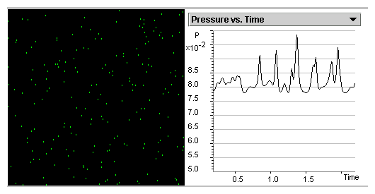
7. Pause the simulation. Switch
Display particles by: Particle Type. Using the
scroll-bar increase the Temperature to T = 2. Press
Start and wait at least 20 time units.
|
| |
| |
As the temperature is increased, the particles leave the liquid state
and become gas as shown in Figure 1.3.
|
| |
|
|
Q1.14: Which phrase best describes what is happening as the
particles begin to fill your container. " The particles are . .
.''
(a) melting
(b) freezing
(c) evaporating
|
|
|
| |
Figure 1.3: A snapshot visualizing the gas state.
| |
8. Switch Iterations Between Displays to 5. Switch
Display Particles by: to Trajectories. Wait 5 time
units. Pause the simulation. Select Take a Snapshot
- Screen. When the dialog box with the Title of the
Picture appears type in: " Gas (T=2)'' and press Ok.
|
| |
| |
You will compare the trajectories of the particles in the
gas state with trajectories of particles in the solid and liquid
states.
|
| |
|
|
Q1.15: What are the differences between the trajectories in the
liquid and gas states? Try to explain why the trajectories are
different.
|
|
|
| |
|
|
Q1.16: Using your snapshot gallery, describe the differences in
the three states of matter in terms of particle motion.
|
|
|
| |
|
|
Q1.17: Describe in drawings and in words how the state of matter
is related to temperature.
|
|
|
| |
| |
9. Switch Iterations between Displays to 100. Select File- Reset
Experiment.
|
| |
| |
You can further investigate
the trajectories of individual particles in the three states
of matter.
|
| |
| |
10. Select Edit - Select Particle
and choose one particle at the center of the solid. Select
Display Particles by: Selected Trajectories and
press Start. After 10 time units, Pause the
simulation. Raise the Temperature to T = 0.4 and press
Start. For approximately 20 time units, observe the changes
in the trajectory of your selected particle. Pause the
simulation and increase the Temperature to T = 2. Press
Start. Watch the trajectory of your chosen particle for
another 20 time units. Press
Pause.
|
| |
| |
You are watching the behavior of
the chosen particle at different temperatures.
|
| |
|
|
Q1.18: Explain the changes observed in the particle trajectory as
the temperature is raised.
|
|
|
| |
| |
11. Select Take a Snapshot -
Screen. When the dialog box with the Title of the
Picture appears, type " Center''.
|
| |
| |
You
will compare this " center'' particle with a particle from the
" edge'' of the solid.
|
| |
| |
12. File -Reset Experiment.
Repeat the step 10 but now select particle from the edge of
the solid.
|
| |
| |
13. Select Take a Snapshot -
Screen. When the dialog box with the Title of the
Picture appears, type " Edge''.
|
| |
|
|
Q1.19: Compare your snapshots " Center'' and " Edge''. Do you see any difference in the
trajectories in the two different cases of initial position. Explain.
|
|
|
| |
END ACTIVITY
1.2 Temperature
What is temperature?
Our computer model is based on the kinetic molecular theory which
predicts that temperature is related to the motion of a large number of
particles that are continually bumping into one another. The
temperature of an object is a measure of the energy of particle motion.
Energy is one of the most important concepts in science because it is
essential to our existence and it cannot be destroyed. The Law of
Energy Conservation is one of the most fundamental in nature and says
that in any process, the total amount of energy is always conserved.
Energy is not at all easy to define because it exists in many forms that
transform into one another in various chemical and physical processes.
In fact, before the development of modern civilization, human beings
knew how to utilize relatively few sources of energy.
Kinetic energy is one form of mechanical energy and is due to the motion
of an object. The kinetic energy of an object depends only on the
object's velocity v and mass m. In mathematical terms, kinetic
energy can be defined by the equation:
|
|
Q1.20:
Rank the following asteroids according to the amount of damage they
would inflict on Earth during a head-on collision: (a) mass m,
velocity v; (b) mass 2m, velocity v; (c) mass m, velocity 2v.
Explain your answer.
|
|
|
| |
According to the kinetic molecular theory the temperature, T, of a
substance is proportional the average kinetic energy of the
particles in the substance, so that:
|
T � (Ek)avg= |
�
�
|
mv2
2
|
�
�
|
avg
|
. |
| (1.2) |
The average kinetic energy of a large number of particles, (Ek)avg
is equal to the sum of the kinetic energies of all the particles divided
by the total number of particles. A typical laboratory sample contains
about 1023 particles.
Our computer model contains, at most, 200
particles.
|
|
Q1.21: Suppose we have a system of only 3 identical particles, each
with mass m=1. The first has a velocity magnitude v1=2, the
second v2=1, and the third v3=4. Compute the magnitude of
the average kinetic energy of this system. (Note: Our model uses
" computer units'' where the particles are not identified as
specific atoms. For exploration of units, see Feature Tour and HandsOn 34:
Computer versus Real Units).
|
|
|
| |
|
|
Q1.22: Now suppose we have a system of only 2 identical particles, each
with mass m=1. The first has a velocity magnitude v1=2 and the
second has a velocity magnitude v2=4. After a purely elastic
collision, the velocity magnitude of the first particle becomes
v1=3. What is the velocity magnitude of the second particle?
|
|
|
| |
|
|
Q1.23: If we increase the temperature, what happens
to the average speed of particles v? What happens to the average
kinetic energy? Explain your answers.
|
|
|
| |
|
|
Q1.24:
Assuming the temperature remains constant, will heavier particles move
faster or slower than lighter particles? Explain
your answer.
|
|
|
| |
|
|
Q1.25: If temperature increases by a factor of 100, by what factor
will the average particle velocity increase or decrease? Explain
your answer.
|
|
|
| |
The temperature equation is based on the average kinetic energies
of all particles. What about each individual particle? Whatever the
temperature of a substance, the movement of its particles will be chaotic
and the range of their constantly-changing velocities can be quite
large. It is important to study the range of velocity values. For
example, in a chemical reaction, usually only the fastest molecules
react when they collide.
BEGIN ACTIVITY
HandsOn
1: Observing Particle Motion in Hot and Cold Water
Nearly fill one beaker with cold water and another with hot water.
Place a drop of food coloring into each beaker near the rim.
|
|
Q1.26: Describe, in drawings and in words, what you think may be
happening at the molecular level.
|
|
|
| |
END ACTIVITY
BEGIN ACTIVITY
SimuLab
2: Velocity Distribution
|
|
Your objective is to:
Investigate the distribution of particle velocities and its dependence
on temperature and mass.
You will be able to:
Explain why, in a system at fixed temperature, particles
have a wide range of velocities.
Contrast the velocity distribution of a gas at low temperature with
a velocity distribution of a gas at high temperature.
Contrast the velocity distribution of heavy particles with the
velocity distribution of light particles.
|
|
|
| |
| |
1. Open SMDPlayer, select Temperature
from the StatesofMatter folder. Press
Play. Read the captions and follow the instructions. Select
File - Quit
|
| |
| |
In the introductory
movie we see that the average kinetic energy of particles
increases with temperature. We also see that velocities of the
majority of particles increases with temperature.
|
| |
| |
2. Open SMD, select the file
Temperature1 in the States of Matter folder. Press
Start
|
| |
| |
Your system represents a high
density gas of 200 green particles at high temperature.
|
| |
|
|
Q1.27: What is the temperature of your system?
|
|
|
| |
| |
Observe the temperature graph. Go to graph panel and
switch the
graph to Kinetic Energies.
|
| |
| |
The green
line represents the average kinetic energy of the green particles.
|
| |
|
|
Q1.28: What is the
average kinetic energy of the green particles?
|
|
|
| |
|
|
Q1.29: Does the kinetic energy graph coincide with temperature graph?
Explain.
|
|
|
| |
| |
3. Switch Display Particles by: to
Absolute Kinetic Energies.
|
| |
| |
The colors of
the particles indicate their kinetic energies in the rainbow
order: red particles have small kinetic energies, violet particles
have large kinetic energies. Observe how the velocities of the
particles (and their color) change as they collide.
|
| |
| |
4. Press Pause. Set Iterations
Between Displays to 50. Select Edit - Select Particles.
Choose Select Particle(s) and click on any particle in the
display window. Press Start.
|
| |
| |
A
white rim will appear around the selected particle. You will
observe changes in the kinetic energy of this particle over
time.
|
| |
|
|
Q1.30: Does the kinetic energy and the velocity of the selected
particle remain constant? Explain.
|
|
|
| |
|
|
Q1.31: Why are the velocities of the particles not equal? Why do the
colors of the particles change? Explain.
|
|
|
| |
| |
5. Set Iterations between Displays to 100.
Switch the graph to Velocity
Distribution.
|
| |
| |
The x-axis of the graph represents
the velocity and the y-axis represents the percentage of particles with that
velocity. At each update of the screen, the computer program measures the
velocities of all 200 particles and adds these values to the
histogram.
|
| |
|
|
Q1.32: Describe what happens to the histrogram of velocities as more and
more velocity updates are taken into account.
|
|
|
| |
| |
6. Wait until the velocity distribution becomes
a smooth curve with a well-defined maximum which usually happens
when the number of velocity updates (# of obs) reaches approximately 10000.
Press Pause and select Take a Snapshot - Graph
and Take a Snapshot - Screen. Type the name of the
picture " T=4,m=1''.
|
| |
| |
You will need these
snapshots to compare the velocity distributions at different
temperatures. This snapshot represents the particles of mass
m=1 and temperature T=4.
|
| |
|
|
Q1.33: Which velocity value corresponds to the maximum of the histogram?
Predict what will happen to the velocity value for the maximum of the histogram as the temperature is lowered to T = 0.25 and T = 1
|
|
|
| |
| |
7. Hit Pause. Using the temperature scroll
change the Temperature to T=0.25, and
repeat Step 6, naming the snapshots
" T=.25,m=1''.
|
| |
| |
8. Change the Temperature to T=1, and
repeat Step 6, naming the snapshot
" T=1,m=1''.
|
| |
|
|
Q1.34: Do the actual positions of the maxima of the velocity
distributions coincide with your predictions in Q.1.33?
|
|
|
| |
| |
9. Enlarge snapshot gallery window
(by dragging bottom right hand corner). Arrange screen shots on top, velocity distributions below screen shot.
|
| |
|
|
Q1.35: Compare the velocity distributions at different
temperatures from the Snapshot Gallery. Explain how they
are similar how they are different.
|
|
|
| |
|
|
Q1.36: Compare the snapshots of the screen at different
temperatures. Relate the range of colors of the particles in the
screen snapshots and the width of the velocity distributions.
|
|
|
| |
| |
10. Select menu item
Edit - Particles. Choose Change all particle(s) to B
and click on the particle screen. You will not see a change in the particles because
they are displayed in Absolute Kinetic energy mode but now you can vary the
particle's mass. Using scroll bar for mass change B particle mass to
4. Set Temperature T=1. Press
Start.
|
| |
| |
We will investigate how the
velocity distribution depends on the mass of the particle. In our
program, only the blue particles have variable mass. Green
particles always have mass m=1. So in order to change a
particle's mass, we have to change the particle type to B.
|
| |
|
|
Q1.37: Predict what will happen to the histogram of particle
velocities when the particles have mass: (a) m=4 and (b)
m=0.1. Predict the positions of the maxima of the velocity
distributions for each case.
|
|
|
| |
| |
11. Repeat Step
6, naming the snapshot " T=1,m=4''
|
| |
| |
12. Change B particle mass to 0.1.
Repeat Step 6, naming the snapshot " T=1,m=0.1''
|
| |
|
|
Q1.38: Compare the velocity distributions for different particle
masses: m=1, m=4, and m=0.1. Explain how they are similar and how
they differ.
|
|
|
| |
|
|
Q1.39: Does the actual position of the maximum of the distribution
coincide with your predictions in Q.1.37? Explain any difference.
|
|
|
| |
|
|
Q1.40: Compare the snapshots of the screen (colors representing kinetic
energies) with the corresponding snapshots of the velocity
distributions. Explain why the colors are the same while the velocity
distributions are different.
|
|
|
| |
END ACTIVITY
1.3 Research Projects
We encourage you to pursue independent research projects. Science moves
forward through research! Try the suggestion below or design your own.
Or, feel free to write an essay using any of the questions throughout
this chapter as inspiration.
BEGIN ACTIVITY
Research
Project 1: States of Matter
See SimuLab 1
Explore how the decreasing of temperature affects the state of
matter. In SimuLab 1, we explored how
the increase of temperature lead to melting and evaporation of a
substance. Is this process reversible? Will the cooling of gas
leads to condensation and then to freezing? Will the process be
as fast as melting and evaporation is if you just watch the movie
StatesOfMatter in the opposite direction, or it will happen in a
different way?
| |
1. Open SMD and select Gas in the
StateOfMatter folder. Decrease the Temperature to
T=0.4. and observe what happens. You have to wait for about 2000
computer time units. To speed up the process, set Iterations
Between Displays to 1000.
|
| |
| |
2. Decrease the Temperature to T=0.25
and observe the process for another 2000 time units.
|
| |
| |
3. Determine the condensation point
temperature (the point at which the gas becomes a liquid) and the
freezing point temperature (the temperature at which the liquid
becomes a solid) by varying the temperature in the appropriate
range and watching the changes in the order and in the motion of
the particles.
|
| |
END ACTIVITY
BEGIN ACTIVITY
Research
Project 2: Velocity Distribution
See SimuLab 3
Test if the velocity distribution depends on the state of matter or the
density of the substance.
| |
1. Open SMD and select Temperature2 in the StateOfMatter folder.
|
| |
| |
You are visualizing a crystal of blue particles surrounded by a gas of
green particles. The crystal does not melt because in this simulation
the blue particles interact much stronger than the green particles.
(See Show Additional Parameters - BB interaction
parameter.
|
| |
|
|
Q1.41: Read the values of the Temperature and B particle
mass and predict if the velocity distributions of B and G
particles will coincide or differ.
|
|
|
| |
| |
2. Change Display particles by to
Absolute Kinetic Energy.
|
| |
| |
Observe that
the colors of particles in the gas and in the crystal are similar.
This means that particles in the crystal and in the gas has the
same average value, hence they have same temperatures. In other
words they are at thermal equilibrium with each other.
|
| |
| |
3. To save computer time, we recommend setting
Iterations Between Displays to 100 or more. Make screen and
graph snapshots.
|
| |
| |
Compare velocity
distributions for particles in the gas and in the crystal using
Velocity Distribution for G and Velocity Distribution
for B graphs and waiting until the velocity distribution for B
and G particles become smooth curves with well-defined maxima.
|
| |
| |
4. Change particle mass to 0.1 and then 10.
Repeat Step 3.
|
| |
| |
Predict the change in the
velocity distributions.
|
| |
| |
5. Restore B particle mass =1. In
the Additional Parameters window, Change Density to
0.8. Repeat Step 3.
|
| |
| |
Predict the changes
in the velocity distributions.
|
| |
| |
6. Increase the Temperature to T=4.
Predict the changes in the velocity distributions. Repeat Step 3.
|
| |
|
|
Q1.42: Compare the snapshots of velocity distributions of B and G
particles with the initial set and explain their differences and
similarities. Do the velocity distributions depend on the density
or state of matter? Explain your answer.
|
|
|
| |
|
|
Q1.43: Compare the snapshots of the screen at different
conditions.
|
|
|
| |
END ACTIVITY
BEGIN ACTIVITY
Research
Project 3: Velocity Distribution II
See SimuLab 3
Investigate whether velocity the distribution depends on
parameters other than temperature and mass of particles.
| |
1. Open SMD, select the file
Temperature2 from the States of Matter
folder.
|
| |
| |
2. Keep mass of particle B and temperature
constant (Heat bath on). Set Iterations Between
Displays to 100 or more. Vary any other parameter in the
Additional Parameters window. For example, change density,
interaction parameters, boundaries, insert piston, introduce
gravity. For each set of parameters obtain smooth velocity
distributions for B and G particles. Make a snapshot of screens
and velocity distribution graphs for different conditions. Be
sure to run the program for each parameter setting long enough so
that the velocity distributions are smooth.
|
| |
|
|
Q1.44: Compare the snapshots of velocity distributions of B and G
particles and explain their differences and similarities. Can you
conclude whether the velocity distributions depend on any
parameter except temperature and mass? Explain.
|
|
|
| |
|
|
Q1.45: Compare the snapshots of the particle screen at different
conditions and try to relate the parameter changes to what you
see.
|
|
|
| |
END ACTIVITY
BEGIN ACTIVITY
Research
Project 4: Velocity Distribution III
See SimuLab
3
Explore how the velocity distribution aquires its shape due to
particles collisions.
| |
1. Open SMD using the default
configuration. Change Display particles by to Absolute
kinetic energy. Set Iterations between Displays to 100. Switch
graph to Velocity Distribution. Press
Start.
|
| |
| |
At the beginning all the particles are
assigned the same velocity magnitude.
|
| |
|
|
Q1.46: As the simulation proceeds,
why does the distribution of velocities differ
from the initial distribution?
|
|
|
| |
END ACTIVITY
BEGIN ACTIVITY
Research
Project 5: Velocity Distribution IV
See SimuLab 3
Explore how two substances in contact reach thermal equilibrium.
| |
1. Open SMD, select the file
Temperature3 from the States of Matter folder. Switch the
Display Particles by to Absolute Kinetic Energies.
Make a snapshot of the screen. Switch Iterations Between
Displays to 100 and Press Start.
|
| |
| |
The temperature of the crystal is much smaller than that of
surrounding gas.
|
| |
|
|
Q1.47:
Watch the graphs of the average kinetic energies of the blue
and the green particles. Explain what you see on the graph and on the screen
from the point of view of molecular kinetic theory.
|
|
|
| |
| |
2. Reset the experiment. Switch the
graph to Velocity distribution. Collect the velocity
distributions for B and G particles for 10000 observations. Make
snapshots of the velocity distributions.
|
| |
| |
3. Switch the graph back to Kinetic
Energies.
|
| |
| |
Wait until the average
kinetic energies of green and blue particles become equal.
|
| |
| |
4. When the system reaches equilibrium, reset
the velocity distribution by switching to No graph and then
to velocity distribution
|
| |
| |
Collect 10000
observations. Make snapshots of the velocity distributions.
|
| |
|
|
Q1.48: Collect the new set of velocity distributions. Compare them to the
previous distributions from Step 2.
Explain what you see from the point of view of molecular kinetic
theory.
|
|
|
| |
Many chemical reactions are accompanied by the formation of a
gas or occur entirely in the gaseous state. Measuring gas
parameters, such as volume and temperature, gives information
about the stoichiometry of the reaction and the energy
transformation that accompany the reaction. The gas parameters
are: pressure, volume, temperature and density. These parameters
do not change independently, but are linked together and described
quantitatively by the gas laws. The idea that gases consist of a
large number of tiny particles moving randomly in all possible
directions provides the modern explanation for the gas laws and is
the foundation of the Kinetic Molecular Theory.
2.1 The Concept of Pressure
It is interesting to note that at times gas sample can behave like
a solid!. For example think of an inflatable mattress and a second
mattress with coil spring. The air in the inflatable mattress
serves the same function as the coils in the second mattress. In
both cases when pressure is applied the mattresses deform (are
compressed). When pressure is removed the mattress returns to
their original shape (volume).
In the following demonstration you will see how air behaves like an elastic
coil spring.
BEGIN ACTIVITY
HandsOn
2: Tire Pump and Coil Spring
You will need:
a bicycle hand pump or a syringe without a needle
a spring.
1. Put your thumb over the nozzle and pump the piston of either
the hand pump or syringe.
|
|
Q2.1: Do you feel any resistance as you push the piston? Try to
explain your observation.
|
|
|
| |
2. Push the pump handle to the lowest possible position and take your hand
off the handle quickly, releasing the piston.
|
|
Q2.2: What happens and how do you explain it?
|
|
|
| |
3. Compress the coil spring.
|
|
Q2.3: Do you feel any resistance? Propose an explanation.
|
|
|
| |
4. Put the piston of the pump to the lowest position, put your thumb over the
nozzle and pull the piston.
|
|
Q2.4: Do you feel any resistance as you pull the piston? Try to
explain your observation. Clue: repeat the experiment without
dosing the nozzle.
|
|
|
| |
5. Expand the coil spring.
|
|
Q2.5: What do you feel? Propose an explanation.
|
|
|
| |
END ACTIVITY
We observed in the preceding HandsOn activity that a gas behaves
much like a coiled spring. If a certain force is applied to the
piston, the volume of a gas under the piston is reduced. If this
force is removed, the gas expands.
In the quantitative study of such elastic properties of the air, one of
the greatest contributions was made in the second half of 17th century
by the Irish chemist Robert Boyle (1627 - 1691). He discovered that
although a force is what is acting on the piston, the amount of force
applied per unit of area is the essential parameter. Boyle was talking
about the concept of pressure. Boyle performed quantitative
experiments to measure the relationship between the pressure and volume
of air.
Pressure is the ratio of the force to area over which it is applied.
Pressure is measured in Pascals. One Pascal equals the pressure created
by a force of one Newton distributed over the area of one square meter. If
you are wondering how much one Pascal is, it is roughly equivalent to the
pressure created by a piece of paper lying on your kitchen table.
When we applied force to solid objects, they deform. However the
magnitude of the deformation depends not on the force, but rather
on the pressure. To reduce the pressure on your shoulders, the
straps of your backpack are made wide. Imagine how uncomfortable
it would be if the straps were made of thin ropes. If the
deformation is not too high, if the force is taken away, the solid
returns to his original shape. The most common example of an
elastic object is a coil spring. Coils springs are used in
mattresses. When you sit down the coil spring shrink, when you
stand up the mattress returns to its original shape.
|
|
Q2.6: Assume the pressure caused by a book balanced on your finger is
P. If you were to balance the same book on your hand (with an area 50
times that of your finger), what would this new pressure be?
|
|
|
| |
|
|
Q2.7:
Calculate the pressure caused by a 1 Kg book if balanced
on your palm (area approximately 1.5 ×10⁻² m2)
vs. the pressure created by this same book balanced on your index
finger (area approximately 3 ×10⁻⁴ m2).
|
|
|
| |
We can conclude from this example that the pressure of a given force
distributed over a small surface is much greater the pressure
distributed over a large surface.
One of the most commonly encountered examples of pressure is that
of the atmosphere. The atmosphere exerts pressure on any object on
the surface of the Earth. Atmospheric pressure at sea level is
101,000 Pascals. This means that the air presses down on 1
square meter surface with the magnitude of 101,000 Newtons,
which is approximately equivalent to the weight of 10,000
kilograms.
The following experiment will allow you to understand
the relative magnitude of atmospheric pressure.
BEGIN ACTIVITY
HandsOn
3: Atmospheric Pressure
|
|
CAUTION:
Do not do this without teacher supervision. Goggles and gloves are
highly recommended.
|
|
|
| |
You will need:
1. Pour two tablespoons of water into a 12 ounce plastic bottle with a screw
cap.
2.
With the cap off, place the bottle into a microwave oven and heat
it until the water starts to boil.
3. Put on your oven mits or winter gloves and remove the bottle from
the microwave. Immediately replace the cap.
4. Put the bottle under
running cold water.
|
|
Q2.8: What do you see and how do you explain it? Clue: In this
experiment the atmospheric pressure remains the same but the
pressure inside the bottle drops when we cool it down.
|
|
|
| |
END ACTIVITY
2.2 Boyle's Law
While performing several experiments, Robert Boyle determined that at
constant temperature the volume of a gas is inversely proportional to the
pressure: V 1/P, or in other words, product of P times V
remains constant when both of these variables change
In this equation, the constant depends on the temperature of the
gas sample and the number of gas particles. The higher the
pressure, the smaller the volume occupied by the gas.
BEGIN ACTIVITY
SimuLab
3: Qualitative Investigation of Boyle's Law
Gas creates pressure because its particles collide with the walls
of their container. The concept of moving gas molecules is the
foundation of the kinetic molecular theory.
|
|
Your objective is to:
Recognize the effect of molecular collisions with the piston on
the piston's position.
You will be able to:
Predict what happens to the position of the piston when the
external pressure is greater than the internal pressure of the
gas.
Explain why the position of the piston fluctuates when the external and
internal pressures are approximately equal.
Describe gas pressure in terms of molecular collisions.
State the relationship between frequency of collision and the volume of a
given gas sample.
|
|
|
| |
| |
1. Open SMDPlayer, select
IntroBoyle'sLaw in the IdealGas folder. PRESS Play.
Read all the captions, and follow the instructions. Go to
File - Quit
|
| |
| |
Movie gives a
preliminary understanding of Boyle's law from a microscopic point
of view.
|
| |
| |
2. Open SMD, select Boyle-Preliminary in the
IdealGas folder.
|
| |
| |
You see 200 green gas molecules under a piston
represented by a red bar, as shown in Figure 2.1. Note
that the Heat Bath is on, which means that the temperature
of the system is kept relatively constant throughout the
experiment. The system is NOT thermally isolated.
|
| |
| |
3. Set Iterations Between Displays to 10. Select Display
Particles by Trajectories and press Start.
|
| |
| |
The particles start to move along straight lines with various
velocities. They change their trajectories when they collide with
the piston or each other.
|
| |
| |
4. Click back to
Display Particles by Particle Type and observe the Volume
versus Time graph.
|
| |
| |
The external pressure acting on the piston accelerates it
downward, reducing the volume of the gas. In the absence of
collisions with the piston, a graph of volume versus time is a
smooth parabola because the piston falls freely. However, when a
molecule collides with the piston, the piston's velocity instantly
changes and the graph as a whole changes into a set of parabolic
segments. The connections of parabolic segments illustrate
numerous collisions that create internal pressure which pushes the
piston upward.
|
| |
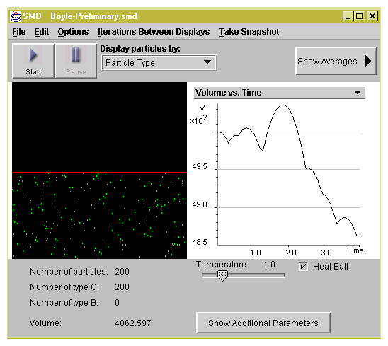 Figure 2.1: Screenshot of Boyle's Law SimuLab.
| |
5. Watch the graph for approximately 4 time units (until the graph
fills the screen) and then press Pause.
To copy the graph to
the " Snapshot Gallery'' select Take Snapshot
:Graph.
|
| |
| |
Determine the number of particle collisions with the
piston by counting the number of parabolic segments as shown in
Figure 2.2.
|
| |
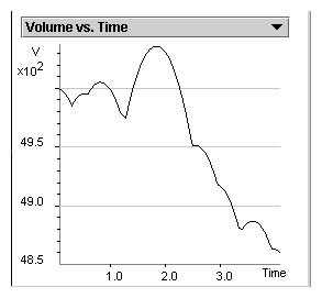 Figure 2.2: Determining the number of molecules collisions with the
piston by counting the parabolic segments. The end of a parabolic
segment is indicated by a jaggedness in the curve. When the number
of parabolic segments is unclear-estimate. In this graph, there
are 7 or 8 collisions (parabolic segments).
Figure 2.2: Determining the number of molecules collisions with the
piston by counting the parabolic segments. The end of a parabolic
segment is indicated by a jaggedness in the curve. When the number
of parabolic segments is unclear-estimate. In this graph, there
are 7 or 8 collisions (parabolic segments).
|
|
Q2.9: How many collisions with the piston (i.e., parabolic
segments) did you count?
|
|
|
| |
| |
6. To speed up the program, set Iterations Between Displays to
1000 and press Start. Run the program for 200 time units
(read Time from Averaging Window).
|
| |
| |
At
equilibrium, the internal pressure created by the gas molecules
colliding with the piston, should be equal to the external
pressure, which is set at 0.04. The internal pressure value can be
found in the Average Values panel. The external pressure value
can be found in the Additional Parameters window by selecting
Show Additional Parameters. Read the volume of the gas from the
Average Values panel and record it. While running this simulation
answer the following questions:
|
| |
|
|
Q2.10: Notice that relatively few particles collide with the piston
at any particular moment. Will this cause the internal pressure
to (a) stay the same, (b) fluctuate a little, or (c) fluctuate
greatly? Explain your reasoning.
|
|
|
| |
|
|
Q2.11: If the external pressure is greater than the internal
pressure, what will happen to the piston?
If the external pressure is less than the internal pressure, what
will happen to the piston?
|
|
|
| |
|
|
Q2.12: If the internal pressure is averaged over an extended
period of time and we wait until the system comes to equilibrium,
will the average internal pressure be (a) higher, (b) lower, or
(c) equal to the external pressure? Explain your reasoning.
|
|
|
| |
|
|
Q2.13: At equilibrium, what happens to the piston?
|
|
|
| |
|
|
Q2.14: What happens to the volume of a gas at equilibrium? Does
this happen in our simulation?
|
|
|
| |
|
|
Q2.15: What role, if any, does the number of particles in our
simulation have on the fluctuations in volume at equilibrium?
|
|
|
| |
|
|
Q2.16: Describe the equilibrium state for a gas contained in a
container with a piston.
|
|
|
| |
| |
7. Press Pause. Double the External Pressure to 0.08.
|
| |
|
|
Q2.17: According to Boyle's Law, predict what should happen to the
average volume when we double the external pressure.
|
|
|
| |
| |
8. Select Reset Averages on the Average Values panel. Press Start.
|
| |
| |
By resetting averages you eliminate the
data from the previous stage of the experiment when the pressure
was 0.04.
|
| |
|
|
Q2.18: Describe what happens to the piston position and explain
why. What happens to the volume of gas?
|
|
|
| |
| |
9. Select the Pressure versus Time graph on the Graph
panel. When the internal pressure value displayed on the graph is
approximately equal to the external pressure, press Pause.
Record the volume of the gas from the main window.
|
| |
| |
You are observing the gas
system approaching equilibrium where the internal and external
pressure are approximately equal.
|
| |
|
|
Q2.19: How does the volume you recorded compare to your prediction?
To what extent are the simulation results consistent with Boyle's Law?
|
|
|
| |
| |
10. Set Iterations Between Displays back to
10. Select the Volume versus Time graph on the Graph panel. Press
Start. Watch the graph for approximately 5 time units (until
graph fills the screen). Press Pause. Copy the graph to the
" Snapshot Gallery'' by selecting Take Snapshot :
Graph.
|
| |
| |
Determine the number of
particle collisions with the piston by counting the number of of
parabolic segments, which represent the number of particle
collisions with the piston.
|
| |
|
|
Q2.20: How do the two graphs compare in terms of the number of parabolic
segments? Propose an explanation for the observed 1 to 2 ratio.
|
|
|
| |
|
|
Q2.21: How does the change in volume relate to the frequency of
collisions with piston?
|
|
|
| |
|
|
Q2.22: How does the change in frequency of collisions relate to the
change in internal pressure?
|
|
|
| |
END ACTIVITY
BEGIN ACTIVITY
SimuLab
4: Quantitative Investigation of Boyle's Law
|
|
Your objective is to:
Test that the product PV remains constant for several positions
of the piston at constant temperature.
You will be able to:
State Boyle's Law.
Construct a P versus V graph from collected data.
Construct a P versus 1/V graph.
Contrast the two curves.
Explain the significance of the slope on the P versus 1/V graph.
Predict what will happen to the PV product if the temperature is
changed.
Construct a P versus number density graph.
Reformulate Boyle's Law in terms of gas density.
|
|
|
| |
| |
1. Open SMD, select Boyle1000 in the IdealGas
folder.
|
| |
| |
You will see 200 particles compressed in a container whose
volume is fixed at 1000. The Temperature is set at 1.25 and
the Heat Bath is on (i. e. the temperature is maintained at
a relatively constant value).
|
| |
| |
The molecules start to move and bump into the walls of the
container. The graph panel represents the internal pressure
created by 200 gas particles at a given moment.
|
| |
|
|
Q2.23: How do you explain the relatively large fluctuations in the
pressure of the system?
|
|
|
| |
| |
Observe the time and the other values
carefully.
|
| |
|
|
Q2.24: Wait for about five time units. Do you notice any change in
the fluctuations of the pressure values in the Average Values
panel?
|
|
|
| |
|
4. Change Iterations Between Displays to 500. Let the program
run for approximately 20 time units. Press Pause.
|
| |
In order to obtain accurate value for
pressure we need to average data over a longer period of time.
Iteration setting of 500 speeds up the simulation.
|
| |
| |
5. Record temperature, number density, volume, and pressure data from
the Average Values panel into the table. Calculate the PV
value.
|
| |
| |
You will need these data for
further analysis.
|
| |
Table I
| Volume | 1000 | 2000 | 4000 | 8000 | 10,000 |
| Temperature | | | | | |
| Number Density | | | | | |
| Pressure | | | | | |
| PV | | | | | |
| Deviation from average | | | | | |
| %
deviation | | | | | |
Calculate (PV)ave value = �i=15 Pi Vi
:________
Deviation from average = | (P V)i - (P V) avg|
% deviation = (|(PV)ave-PiVi|)/((PV)ave) x 100
Calculate average % deviation = �i=15(|(PV)ave-PiVi|)/((PV)ave) x 100
value:________
| |
6. Select File : Open Preset Experiment and open
Boyle2000. Press Start. After approximately 20 time
units press Pause. Record the values and calculate the PV
value as described in Step 5.
|
| |
| |
In
order to test Boyle's law, we will measure the pressure of the
same amount of gas at the same temperature and different
volumes.
|
| |
| |
7. Repeat Steps 6 for Boyle4000, Boyle8000, and
Boyle10000.
|
| |
|
|
Q2.25: Compare the values of PV for various volumes. Find the
average value of these products and calculate the deviation of
each PV value from the average. Calculate the percent deviation
of each ( PV) i value from the average (PV) ave by using this formula:
|
%deviation = |
�
�
|
| (PV)i-(PV)ave|
(PV)ave
|
×100 |
�
�
|
|
|
Find the largest percent deviation.
To what extent are your results consistent with Boyle's Law?
Hint: Refer to your percent deviation and range of values of
pressure.
|
|
|
| |
|
|
Q2.26:
Construct a Pressure vs. Volume graph.
This plot represents the dependence of pressure on volume
at constant temperature. According to Boyle's law, when the
temperature is constant, the graph should be a hyperbola.
If your graph varies significantly from a hyperbola, do you
have any idea why this may have been so?
|
|
|
| |
|
|
Q2.27:
Construct a Pressure vs. 1/Volume graph. Draw the line of best
fit through the data points. Determine the slope of this line and
compare it to the average PV product in the above chart.
What is the relationship between the slope and the average PV
product?
What is the difference between the graph of P vs. 1/V and
the graphs of P vs. V graph?
|
|
|
| |
|
|
Q2.28: Construct a Pressure vs. Number Density graph. Number
Density is defined as Number of particles over volume: n = N/V. The distribution of data points should fall as a
straight line.
What is the relationship between pressure and number density?
Compare this graph to the Pressure vs. 1/Volume graph. We
should now be able to state an alternative form of Boyle's law:
at constant temperature, the gas pressure is directly
proportional to the gas number density.
|
|
|
| |
|
|
Q2.29:
Find the slope of the Pressure vs. Number Density
graph and comment on the relationship between the slope and temperature of
the system.
|
|
|
| |
|
|
Q2.30: Graph the PV product vs. Pressure.
What slope do you expect? What do you find? Explain the deviation from
your prediction (Hint: consider that ideal gas behavior is followed at
low pressures and high temperatures).
|
|
|
| |
END ACTIVITY
2.3 Temperature
BEGIN ACTIVITY
HandsOn
4: The Subjective Sensation of Temperature
1. Label three bowls each half-filled with hot (roughly 500C) water
as 1, 2, and 3.
2. Fill the bowl 1 with hot water (roughly 400 C) and bowl
3 with cold water (roughly 200 C). Pour 1/3 of water from
bowl 1 and 1/3 from bowl 3 into bowl 2 and stir.
3.
Immerse your left hand into bowl 1 and your right hand into bowl 3. Let
your hands stay there for a minute. After you've done that, take them
out and immerse both of your hands into bowl 2.
|
|
Q2.31: Is water in the middle bowl hot or cold? Explain.
|
|
|
| |
From this simple experiment, you have hopefully discovered that
the hand is not an accurate thermometer. Galileo observed that
almost all substances expand when they are heated.
This insight led to the construction of the first thermometer.
END ACTIVITY
BEGIN ACTIVITY
HandsOn
5: HandsOn: Galileo's Thermometer
We can try to duplicate Galileo's thermometer with the aid of everyday
household items.
You will need (as shown in Figure 2.3):
a small glass or plastic bottle
a cork that fits the bottle
a thin glass tube about 10 inches long (you can use a transparent
plastic straw if you do not have a glass tube)
a drill with drill bit slightly smaller than the diameter of the tube
Figure 2.3: Schematic of Galileo's Thermometer experiment.
1. Drill a hole in the cork and slide the tube through until 0.5
inch. of the tube appears on the other side of the cork, ensuring
that there is a tight fit. If the fit is not so tight, remove the
tube and wrap some plastic wrap or Parafilm around the tube and
reinsert.
2.
Remove the straw and cork from the bottle. Carefully dip 0.5 inch
of the tube below the cork into a cup of coffee or cooking oil and
cover the upper end of the straw using your finger so that 0.5
inch of liquid stays in the straw when you take it out.
3. Insert the end of the cork into the bottle so that the top of the
0.5 inch of liquid is even with the top of
the cork. Hold the bottle tightly in your hand.
|
|
Q2.32: What happened to the plug of liquid?
|
|
|
| |
4. Mark your straw every 0.5 inch. You have invented your own temperature
scale, where room temperature corresponds to zero and the temperature of
your hands to, for example, ten. You can assign your own values to your
thermometer since you invented it! Notice that your thermometer does
not have a wide temperature range.
|
|
Q2.33: How would you increase the temperature range of your thermometer?
|
|
|
| |
END ACTIVITY
BEGIN ACTIVITY
SimuLab
5: Galileo's Thermometer - Movie
Due to the small number of particles in our system it would
take a very long time for a liquid droplet in a tube to reach
thermal equilibrium. To reduce the time of this activity, we will
explore a movie of the simulation.
|
|
Your objective is to:
Understand the principle of how a thermometer works in terms of
molecular motion.
You will be able to:
Explain how a thermometer works in terms of molecular motion.
Explain why the column of liquid goes down as temperature is
decreased.
|
|
|
| |
| |
1. Open SMDPlayer, select Galileo-Thermometer in the
IdealGas folder. Press Play.
|
| |
| |
The movie pauses at the opening
frame and displays the first explanatory caption. In order to
better visualize the particles, you can select Edit
: Background White. The narrow column on the screen represents
our thermometer tube, blue particles represent air molecules, and
the green layer represents a liquid droplet.
|
| |
| |
2. Press Play to resume the movie. The movie pauses at each
explanatory caption. Repeat this step until the end of the movie
is reached.
|
| |
| |
At a given temperature,
the droplet fluctuates around a certain equilibrium position. Each
time the temperature drops in our simulation, the equilibrium
position of the green layer also drops. Near the end of the
movie, we simulate the effect of the thermometer inserted into an
extremely hot environment: everything is thrown out of the tube
and your thermometer breaks!
|
| |
|
|
Q2.34: Describe the relationship between the height of the gas
sample and the temperature. Explain how the thermometer works in
terms of molecular motion.
|
|
|
| |
END ACTIVITY
2.4 Charles Law
A century after Boyle derived his law, the French scientist
Jacques Charles (1746 - 1823) discovered a linear relationship
between gas temperature and gas volume when pressure is kept
constant. Using a temperature versus volume graph, he discovered
that the volume of any gas at constant pressure would approach
zero at -2730C. He did not publish these results. Twenty years
later, another French chemist, Joseph Gay-Lussac, repeated
Charles' experiments, got the same results, and published them. At
that time, however, no one could even get close to -2730C in a
laboratory, so Gay-Lussac could only determine his law by
extrapolating the volume line on his graph until it crossed the
temperature-axis. Later, this temperature was called absolute
zero. The name for the new temperature scale, which has the origin
at absolute zero, is the Kelvin scale. Zero degrees in Kelvin
corresponds to -2730C and is the temperature at which all
molecular motion ceases.
In the next simulation we will demonstrate Charles' Law from a
microscopic point of view. We will put a gas in a cylinder under a
piston and keep the external pressure constant. Imagine that this
pressure is created by a constant weight resting on top of the
piston. At any given temperature, the particles have a certain
average velocity. They collide with the piston and the walls of
the cylinder, thus, causing pressure. If the temperature is
lowered, the average velocity of the particles decreases, and the
particles collide with the piston and cylinder walls less
frequently and with less force and thus the internal pressure
drops. Since the weight resting on top of the piston remains
constant, the piston descends until the pressure inside the
cylinder becomes equal to the external pressure, therefore
reaching equilibrium again. As the volume of the gas decreases the
number of collisions with the walls increase and thus the internal
pressure increases. Since we only have 200 particles in this
simulation, there are relatively few collisions with the piston,
and the piston constantly moves up and down. In a real experiment,
with 1023 or more molecules in a sample, the drumming on the
piston produced by such a great number of molecules is constant
and would not lead to macroscopic oscillations, and the piston,
after a few initial initial oscilations stays almost constant.
BEGIN ACTIVITY
SimuLab
6: Charles' Law - Movie
|
|
Your objective is to:
Recognize the microscopic origin of the volume variations with
temperature at constant external pressure.
You will be able to:
State Charles' Law.
Construct a volume versus temperature graph from collected data.
State the relationship between volume and temperature.
Determine the temperature at which the volume would be zero and
explain the significance of this point.
Propose reasons as to why the V/T value deviates from
predictions of Charles' Law.
State the relationship between number density and temperature.
|
|
|
| |
| |
1. Open SMDPlayer, select Charles in the IdealGas folder. Select Show
Averages. Press Play to resume the movie. The movie pauses
at each explanatory caption. Follow the instructions in each
caption, making sure to Reset Averages in the Average Values
panel. Repeat this step until the end of the movie is reached. If
you wish to see the temperature in Kelvin scale press Real
Units button.
|
| |
| |
Notice that the average pressure stays approximately the
same throughout the entire movie. Note that the temperature
throughout the movie decreased by a factor of 2.5. In our
simulation, the temperature of the gas sample is equal to the
average kinetic energy of the molecules. The average kinetic
energy is proportional to the average velocity squared (Ek=( (mv2)/2) avg). Therefore, the
average velocity is decreased by �{2.5} � 1.6. Did you
notice that the particles move slower at the end of the movie than
at the beginning? To compare, you can watch the movie
again.
|
| |
Deviation from average = |( V/T)i -( V/T)ave|
% Deviation = (|( V/T)i -( V/T)ave|)/(( V/T)avg) ×100
|
|
Q2.35: Plot Volume vs. Temperature on a graph. Draw a line of best
fit through the points.
|
|
|
| |
|
|
Q2.36: What is the relationship between volume and temperature?
|
|
|
| |
|
|
Q2.37:
On a Volume vs. Temperature graph, for an ideal gas the line
intersects the temperature axis at the origin. Comment on the extent to
which your graph is consistent with Charles' Law.
|
|
|
| |
|
|
Q2.38:
Compare the values of V/T for various temperatures. Find the
average value of these ratios and calculate the deviation of each V/T
value from the average. Calculate the percent deviation of each
( V/T) i value: and calculate the average percent deviation.
|
|
|
| |
|
|
Q2.39: Plot the Number density vs. Temperature graph.
|
|
|
| |
|
|
Q2.40: How does number density vary with temperature?
|
|
|
| |
END ACTIVITY
2.5 Gay-Lussac Law
Joseph Gay-Lussac (1778-1850) continued investigating gases and
performed an experiment in which he changed the temperature and
kept the volume constant. He found that at constant volume the
pressure increases linearly with temperature. The graph of
pressure vs. temperature is a straight line. The slope of this
line depends on the volume of the gas sample and on the number of
gas particles. For various volumes the lines, when extrapolated,
cross approximately at the point P = 0, T = -2730C on the
graph. This point corresponds to the same temperature as in the
Charles' Law graphs where pressure was held constant. At this
temperature the gas exerts no pressure at all. Later this
temperature was called absolute zero, and a new temperature scale
called Kelvin was established. Zero degrees Kelvin, corresponds to
-2730C. Gas pressure is created by collisions of particles with
the walls, therefore at absolute zero the particles of gas should
completely stop moving. In terms of the Kelvin temperature scale,
the Gay-Lussac law can be written as
where the constant depends on the volume and the number of gas particles.
BEGIN ACTIVITY
SimuLab
7: Gay-Lussac Law
|
|
Your objective is to:
Recognize the microscopic origin of the internal pressure
variations with temperature at constant volume.
You will be able to:
State Gay-Lussac's Law.
Construct a Pressure vs Temperature graph.
Extrapolate the slope on the graph to P=0 and explain the
significance of this point.
Determine the temperature range at which data is consistent with
Gay-Lussac Law.
Suggest reasons why deviations from Gay-Lussac Law occur.
|
|
|
| |
| |
1. Open SMD, select Gay-Lussac in the IdealGas
folder.
|
| |
| |
You see 200 gas molecules
in a fixed volume, the temperature is T = 4.0 and the Number
Density ( N/V) = 0.02 (number of particles
divided by volume).
|
| |
| |
2. Select Show Averages.
Press Start. Watch the Pressure vs. Time graph for
approximately 5.0 time units.
|
| |
| |
You
can see that the fluctuations of pressure are rather significant
and the values on the Average Values panel are constantly
changing. In order to obtain accurate measurements, you need to
average data for significantly longer times, such as 20 time
units.
|
| |
| |
3. Change Iterations Between Displays to 500. Let the program
run for approximately 20 computer time units as shown in figure
2.4. Press Pause.
|
| |
| |
Setting Iterations Between Displays at 500
speeds up the simulation.
|
| |
Figure 2.4: Screenshot of Gay-Lussac's Law SimuLab.
| |
4. Record the pressure from the Average Values panel for this trial
in your Table for T=4. Calculate the P/T value. Press
Reset Averages on the Average Values panel.
|
| |
| |
You are preparing data for the future
analysis.
|
| |
| |
5. Set the Temperature to T=3. Press Start. Let the
program run for 20 time units. Press Pause. Record
Pressure and calculate P/T ratio. Select Reset Averages
on the Average Values panel.
|
| |
| |
Ressetting
Averages allows you to delete the data values from the previous
experiment.
|
| |
| |
6. Repeat Step 5 for Temperatures T=2, T=1.25,and T=1.
|
| |
|
|
Q2.41:
Compare the values of P/T obtained for various temperatures with the
average value of P/T from the table. | ( P/T)i - ( P/T )avg |.
Express the differences in percents
|
|
|
|
�
�
|
�
�
|
P
T
|
�
�
|
i
|
- |
�
�
|
P
T
|
�
�
|
avg
|
�
�
|
|
|
×100 |
|
and record them into the table.
|
|
|
| |
|
|
Q2.42: What conclusions can you draw about the consistency of
the P/T constant in relation to temperature?
|
|
|
| |
|
|
Q2.43:
Plot a Pressure vs. Temperature graph. Approximate it by a straight
line. Determine the slope of the graph. Extrapolate the line to P=0.
|
|
|
| |
|
|
Q2.44: What is the temperature when P=0? Explain your result.
|
|
|
| |
END ACTIVITY
END ACTIVITY
2.6 Avogadro's Law
In 1809, Gay-Lussac performed several experiments with reacting
gases showing that under constant conditions of pressure and
temperature, volume was not necessarily a conserved quantity. In
other words, if you start out with three volumes of gas, you won't
necessarily end up with three volumes at the end of a chemical
reaction; mass is conserved in a chemical reaction, volume
is not. For example, if two volume units of hydrogen gas
are mixed with one volume unit of oxygen gas at constant pressure,
the water vapor produced by the reaction occupies two volume
units
|
2H2( gas) +O2( gas) � 2H2O(gas). |
|
In this example, the number of atoms (i.e., mass) is conserved on
each side of the equation but the volume of gas is not conserved.
Two years later Italian scientist Amadeo Avogadro (1776-1856)
explained these results by stating that in equal volumes of
any gas at the same temperature and pressure there are equal
numbers of particles. The name of the unit that represents a
certain fixed number of particles is a mole. One mole
contains the Avogadro number NA of molecules, NA=6.02·1023. Then we can reformulate the Avogadro law: at
constant temperature and pressure the volume of gas is
proportional to the number of moles of gas particles:
Remembering that molecular collisions with the sides of a
container cause pressure, then for a chemical reaction performed
in a container of constant volume the Avogadro law gives: at
constant temperature and volume the pressure is proportional to
the number of moles of gas.
BEGIN ACTIVITY
SimuLab
8: Avogadro's Principle
|
|
Your objective is to:
Recognize the role of the number of moles (here the number of
particles) in the determination of the internal pressure of a gas.
You will be able to:
State the relationship between the number of particles and the volume
they occupy if pressure and temperature remain constant.
Calculate the volume when temperature and pressure remain constant.
State Avogadro's hypothesis.
Contrast number density to mass density.
Predict what happens to each parameter if the number of particles is
doubled.
|
|
|
| |
Copy the table below.
| T | P
| V | N (#
of particles) | mass
|
| Avogadro40 | | | | | |
| Avogadro200 | | | | | |
| Avogadro100 | | | | | |
| Avogadro100 | | | | | |
| |
1. Open SMDPlayer, select
IntroAvogadro'sLaw from the Ideal Gas folder. PRESS
Play. Read all the captions and follow the instructions. Go to
File - Quit
|
| |
| |
Movie gives a
preliminary understanding of Avogadro's Principle from a
microscopic point of view.
|
| |
| |
2. Open SMD, select Avogadro40 in the IdealGas
folder. In order to better visualize the particles, you can
select Edit : Background White. To speed up the simulation,
change the Iterations Between Displays to 1000. Select
Show Averages.
|
| |
| |
In this experiment you are visualizing 40 particles (displayed as a B
particle type), each of which has a mass of 1.0 unit.
|
| |
| |
3. Press Start. Observe the Pressure versus Time graph
for approximately 40 time units as shown in figure
2.5. Press Pause.
|
| |
| |
The gas is approaching equilibrium. The pressure fluctuates around an average value.
|
| |
Figure 2.5: Screenshot of Avogadro's SimuLab.
| |
4. Record the temperature T, pressure P, volume V, number of
type B particles N, and the B particle mass
m.
|
| |
| |
You are collecting data for
future analysis and recording it in the first row of the data
table.
|
| |
| |
5. Open Avogadro200 by selecting File - Open Preset
Experiment.
|
| |
| |
In this experiment
you are visualizing 200 particles of mass 1.0. Note that the
piston is now above the screen and you can not see it.
|
| |
| |
You are collecting data for future
analysis and recording it in the second row of the data table.
|
| |
|
|
Q2.45:
Are there any changes in parameters other than the number of
particles? If so, what are they?
|
|
|
| |
|
|
Q2.46:
What is the relationship between the number of particles and
the volume they occupy if pressure and temperature remain the same?
|
|
|
| |
|
|
Q2.47: What do you predict the volume to be if you have 100
particles, each with a mass of 1.0?
|
|
|
| |
| |
7. Open Avogadro100 by selecting File - Open Preset
Experiment.
|
| |
| |
This simulation
contains 100 particles of mass 1.0.
|
| |
| |
You are collecting data for
future analysis and recording it in the third row of the data
table.
|
| |
|
|
Q2.48: Speculate: What do you think will happen if we increase the
mass of the particles? Why? To test your speculation, move onto
the next steps.
|
|
|
| |
| |
9. Select File - Reset Experiment. Set B particle mass
to m=10.
|
| |
| |
Now this simulation
contains 100 particles of mass 10.0.
|
| |
| |
10. Repeat Steps 2 and 3.
|
| |
| |
You are collecting data for
future analysis and recording it in the fourth row of the data
table.
|
| |
|
|
Q2.49: What happened to the parameters of temperature, pressure,
and volume when you changed the mass of the particle?
|
|
|
| |
|
|
Q2.50: In our simulations, " density'' always refers to number
density N/V. The density which you are probably most
familiar with is mass density M/V= mN/V; where M is
mass, V is volume, m is mass of a single particle and N is
the number of particles.
What happens to the number density when the B particle is set to a
mass of m=10 in Step 7?
|
|
|
| |
|
|
Q2.51: What happens to the mass density when the B particle is set to
mass m=10? Contrast this to the Number Density above and explain.
|
|
|
| |
|
|
Q2.52: What do you predict the volume would be for 175 particles of Mass=5?
|
|
|
| |
|
|
Q2.53: Consider two 1-liter balloons at room temperature. One
balloon is filled with one mole of He gas and the other with one
mole of Ne gas. How do their pressures, mass densities, and number
densities compare?
|
|
|
| |
END ACTIVITY
BEGIN ACTIVITY
SimuLab
9: Avogadro's Principle Movie
|
|
Your objective is to:
Investigate the relationship between the number of gas particles
and the volume they occupy if temperature and pressure are kept
constant.
You will be able to:
State the relationship between the number of particles and
the volume they occupy if pressure and temperature remains
constant.
State Avogadro's hypothesis.
Contrast mass density with number density.
Explain the relationship between volume, number density and
mass density in terms of Avogadro's Principle.
|
|
|
| |
| |
1. Open SMDPlayer, select Avogadro in the IdealGas
folder.
|
| |
| |
You see a mixture of gases
under a piston. Follow the instructions in the captions.
|
| |
| |
2. Press Play. The movie pauses at the opening frame and
displays the first explanatory caption. Select Show
Averages. The movie pauses at each explanatory
caption.
|
| |
| |
The Averages panel displays
average (not instantaneous) values of the parameters as the
experiment proceeds.
|
| |
| |
3. Press Play to resume the movie after each caption. Be sure
to reset Averages when instructed to do so thus eliminating
data from previous setting.
|
| |
|
|
Q2.54: What has happened to the total number of particles as the
product molecules are formed?
|
|
|
| |
|
|
Q2.55: If the temperature and the pressure of the system are kept
constant, what will happen to the volume as the number of gas
particles decreases?
|
|
|
| |
|
|
Q2.56: What happened to the mass density of the gas? Explain.
|
|
|
| |
|
|
Q2.57: What happened to the number density? Explain.
|
|
|
| |
|
|
Q2.58: Explain the changes in volume, number density, and mass density in
terms of Avogadro's Principle.
|
|
|
| |
END ACTIVITY
2.7 Ideal Gas Law
We arrive at the gas state equation by combining Boyle's Law,
Charles' Law, Gay-Lussac's Law, and Avogadro's Principle:
where k=1.38·10-23J/K is the Boltzmann constant and N
is the number of particles in the gas. Usually we use moles
instead of number of particles, because the number of particles is
huge in typical laboratory gas samples while the numbers of moles
have reasonable values. In a mole there is the Avogadro number
NA of molecules. If the number of moles in the gas sample is
n, then N=NA n is the number of particles. If we define
R=kNA we can rewrite the gas equation as:
or
where R=8.31J/(K·mole) is the so called universal gas
constant and n is the number of moles of gas. The above
equation is called the ideal gas law. It is valid only if
the gas possess " ideal'' properties:
An Ideal gas is not real, but rather a hypothetical
substance. Real gas molecules, however, do have a tiny
volume and do interact with each other. Therefore there are
always deviations from the Ideal Gas Law. When conditions are
close to " ideal'' (i.e., at low pressures and high temperatures)
the deviations are very small. Often, though, conditions are
" less than ideal''. This occurs when any of the ideal gas
properties above fails to be true. For example, at low
temperatures we can not neglect the interaction between the
molecules which lead to phase transitions.
|
|
Q2.59: What kind of virtual experiment would you perform to
determine if you are modeling a real or ideal gas?
|
|
|
| |
END ACTIVITY
BEGIN ACTIVITY
SimuLab
10: Ideal Gas Law
|
|
Your objective is to:
Test the ideal gas law by obtaining V, T and P measurements
and evaluating the consistency of the PV/NT ratio at
various conditions.
You will be able to:
Test the validity of the ideal gas law at low densities and high
temperatures.
Define the Boltzmann constant.
Test that the ideal gas law is valid for various molecular masses.
Find the limits of the ideal gas law in terms of gas density and
temperature.
|
|
|
| |
| |
1. Open SMD, select IdealGasLaw in
the IdealGas folder. To better visualize the particles,
select Edit: Background Gray.
|
| |
| |
You are visualizing a gas mixture that consists of 100 green and
100 blue particles as shown in figure 2.6. You will
perform three experiments (set ups A, B and C).
|
| |
Figure 2.6: Screenshot of the Ideal Gas Law SimuLab.
| |
2. Set Iterations Between Displays to 1000. Select Show
Averages.
|
| |
| |
Higher number of
Iterations Between Displays speeds up the program.
|
| |
| |
3. Press Start and wait for approximately 20 time units. Press
Pause. Record temperature T, pressure P, volume V,
number of particles N (set-up A in your table). Calculate number
density N/V and PV/NT.
|
| |
| |
The system has reached the equilibrium and you are
collecting data for further analysis.
|
| |
Table I
Set-up A: 100 green particles, 100 blue, mass = 1
Set-up B: 100 green particles, mass = 1
Set-up C: 100 blue particles, mass = 10
| |
4. Select File - Reset Experiment.
Select Edit - Particles and choose Remove all B
particles (blue particles) and click on the display window to
take this action. Select Reset Averages in the Average
Values panel. Repeat Step 3, using set-up B in your
table.
|
| |
| |
Resetting Averages eliminates the data from previous experiments. You are now collecting
data for this experiment.
|
| |
| |
5. Select File - Reset experiment.
Select Edit - Particles and choose Remove all G
which removes all green particles. Set the
B particle mass to 10. Select Reset Averages in the
Averages Values panel. Repeat Step 3 using set-up C in your table.
|
| |
|
|
Q2.60:
Compare the values of PV/NT found in set-ups
A, B, and C. Calculate the average value which represents the Boltzmann
constant in computer units.
Theoretically, the Boltzman constant is 1.0 in our computer
simulation. In set-up A the gas density is 0.02 and is too high to
give the theoretical value. In set-up B and C, the gas density is
0.01 and approaches ideal behavior.
|
|
|
| |
Now we will determine the range of densities for which the ideal gas
law equation is valid.
| |
6. Select File - Reset experiment. Select Edit - Particles and choose
Change all particles to G (making all
particles green).
|
| |
| |
You are preparing experimental set-up D.
|
| |
| |
7. Select Show Additional Parameters. Using scroll bar and / or arrow key,
set Number Density to 0.1. Press
Start. Wait approximately 10 time units so that equilibrium is
reached.
At this point, Reset Averages in the
Average Values panel and wait another 20 time units. Press
Pause. Record parameters in your table and compute N/V and
PV/NT.
|
| |
| |
You are watching the approach to equilibrium and collecting data for set-up D
when equilibrium has been
reached.
|
| |
Table II
Set-up D: 200 green, N/V=0.1
Set-up E: 200 green, N/V=0.2
Set-up F: 200 green, N/V=0.5
|
|
Q2.61: How does your ratio PV/NT compare to the
theoretical value of 1.0?
|
|
|
| |
| |
8. Repeat Step 7 for Number Density 0.2 and 0.5.
|
| |
| |
You are collecting data for set-ups E and F.
|
| |
|
|
Q2.62: Comment on the consistency of the PV/NT ratio as
number density of the gas increases.
|
|
|
| |
Now we will determine the
range of temperatures for which the ideal gas law equation is valid.
| |
9. To configure setup G : set Number Density to 0.02.
|
| |
| |
You are creating a very low density gas. You can choose the option " distribute particles instantaneously'' to save time.
|
| |
| |
10. Set Temperature to 2. Press Start. Wait approximately
10 time units so that equilibrium is reached. At this point,
Reset Averages in the Average Values panel and wait another 20
time units. Record parameters in your table and compute
PV/NT in the data table.
|
| |
| |
You are collecting data
for set-up G. Resetting Averages eliminates data from when the
system was not yet at equilibrium.
|
| |
Table III
Set-up G: 200 green, T=2
Set-up H: 200 green, T=1
Set-up I: 200 green, T=0.5
| |
11. Repeat Step 10 for temperatures 1 and 0.5.
|
| |
| |
You are collecting data
for set-up H and I.
|
| |
|
|
Q2.63: How consistent is the PV/NT ratio when the
temperature is varied in set-ups G, H, and I? Comment on conditions necessary for ideal gas behavior.
|
|
|
| |
END ACTIVITY
Consequences of the Ideal Gas Law
When a gas is compressed at constant temperature, the gas
particles have less space to move around. They collide with the
walls more frequently, and the internal pressure increases in
accordance with Boyle's law: PV=const.
When we decrease temperature at constant volume, the velocity of
the particles decreases. If the volume is kept constant, they
collide less frequently and exert less force on the walls of the
container. This is consistent with Gay-Lussac's law: P/T=const. At absolute zero the particles have a velocity of
zero, they do not collide with the walls of the container, and the
internal pressure is zero.
If the external pressure is kept constant and the temperature is
lowered, the volume of the gas decreases. At the lowered
temperature, the molecules move slower, therefore collide less
frequently. As a result, the internal pressure decreases. Since
the external pressure is constant, the gas volume decreases until
the number of collisions results in an internal pressure which is
equal to the external pressure. We are assuming that gas particles
have no volume and the pressure is only generated by collisions
with container walls. We also assume that the volume of a gas will
reach zero at absolute zero. This is consistent with Charles' law:
V/T=const.
When we increase the number of particles and keep temperature and
external pressure constant, the number of collisions increases and
the gas expands. This is consistent with Avogadro principle for
the case when P is constant and T is constant: V/n=const. When V is constant and T is constant we obtain
P/n=const.
A mole of any gas at standard temperature and pressure (STP), i.e.
00C temperature and pressure of 1 atm, occupies
RT/P= 8.31 ×273/101,000 = 0.0224 m3=22.4
liters. The universal gas constant is commonly measured in the
units of R=0.082 liters × atm/Kelvin × mole or 8.351J/Kmol.
2.8 Dalton's Law
Until this point, the assumptions of the ideal gas model
effectively provided the prediction of the gas behavior at low
densities and high temperatures. We can try to extend the model
in order to predict the pressure produced by a mixture of
various molecules. Since we define molecules as noninteracting
particles of zero volume, all of them would move in the container
independently. They would collide with the walls and produce
pressure. The molecules of a particular kind cause a pressure that
is unaffected by the presence (or absence) of other molecules.
This is called the partial pressure of that gas. The
molecules of another kind would produce its own partial pressure,
and so on. Then the total pressure in the container is the sum of
all these partial pressures. This statement is known as
Dalton's Law of Partial Pressures:
where P is the total pressure, and P1 and P2 represent the partial
pressure of Gas 1 and Gas 2.
BEGIN ACTIVITY
SimuLab
11: Dalton's Law
In our simulation it is more convenient to use number of particles instead
of number of moles. Moreover, in the simulation units the Boltzmann constant
k=1. Hence, the partial pressures
where Ni is just
a number of molecules of certain type.
|
|
Your objective is to:
Recognize why the total pressure of the gas mixture is equal to
the sum of partial pressures of the components from the
microscopic point of view.
You will be able to:
State Dalton's Law.
State the relationship between the number of particles and pressure they
exert at constant temperature and volume.
Calculate the final pressure as the number of particles are varied when
the initial pressure and number of particles are given.
|
|
|
| |
Copy the table below.
| N/V | P | T
|
| 100 Blue and 100 Green | | | |
| 100 Blue | | | |
| 100 Green | | | |
| |
1. Open SMDPlayer, select
IntroDalton'sLaw from the IdealGas folder. PRESS
Play. Read all the captions and follow the instructions. Go to
File -Quit
|
| |
| |
Movies gives a
preliminary understanding of partial pressures from a microscopic
point of view.
|
| |
| |
2. Open SMD, select Dalton in the IdealGas
folder.
|
| |
| |
You are visualizing 100
green particles with a mass of 1.00 and 100 blue particles each
with a mass of 10.0 as shown in Figure 2.7.
|
| |
Figure 2.7: Screenshot of Dalton's Law SimuLab.
| |
3. Change the Iterations Between
Displays to 500. Select Show Averages.
|
| |
| |
Increasing Iterations speeds up the
simulation.
|
| |
| |
4. Press Start and run the simulation
for approximately 40 time units. Press Pause. Record in
your table the number density N/V, pressure P and
temperature T from the averaging window.
|
| |
| |
The system is approaching equilibrium.
|
| |
| |
5. Select Edit : Edit Particles and choose Remove all
G particles. Press Reset Averages in the Average Values
panel. Repeat Step 4. Note that the blue particles have a mass of
10.
|
| |
| |
You are are
collecting data for future analysis.
|
| |
| |
6. Select File : Reset Experiment. Select
Edit : Edit Particles and choose Remove all B
particles. Repeat Step 4. Note that the green particles have a
mass of 1.
|
| |
| |
7. Using the data recorded in your table, add the pressure of the 100
blue particles to that of the 100 green particles
|
| |
| |
You are summing partial gas pressures.
|
| |
|
|
Q2.64: Compare this calculated result to the total pressure of the
mixture when both blue and green particles were present. Explain what you
find.
|
|
|
| |
|
|
Q2.65: Does the mass of a particle affect the pressure it exerts?
Justify your answer.
|
|
|
| |
|
|
Q2.66: What is the relationship between the number of particles
present and the pressure they exert in a given container?
|
|
|
| |
| |
8. Select File : Reset Experiment. Select Edit : Edit
Particles and choose Remove particles to remove any 20
particles on the screen.
|
| |
| |
You are lowering the density.
|
| |
|
|
Q2.67: What do you predict the pressure will now be?
|
|
|
| |
| |
9. Select Reset Averages in the Average Values panel. Press
Start and wait for 40 time units. Press Pause.
|
| |
| |
The system is approaching equilibrium.
|
| |
|
|
Q2.68: Verify your pressure prediction.
|
|
|
| |
END ACTIVITY
2.9 Research Projects
Try one of the suggestions below or design
your own. Or, feel free to write an essay using any of the questions
throughout this chapter as inspiration.
BEGIN ACTIVITY
Research
Project 6: Boyle's Law
See SimuLab 7
.
To further investigate the universality of Boyle's law, test it for various
temperatures. Set T=1.25, 1.5, 2, 4 and repeat steps 6-8 (in
SimuLab 7 for each temperature value.
|
|
Q2.69: What happened to the PV product when the temperature
increased? Explain.
|
|
|
| |
|
|
Q2.70: At low pressures what is the temperature range in
which the data is most consistent with Boyle's law?
|
|
|
| |
BEGIN ACTIVITY
BEGIN ACTIVITY
Research
Project 7: Gay-Lussac Law
See SimuLab 13.
To extend the SimuLab, repeat Step 6 with N/V=0.10.
| T=4 | T=3 | T=2 | T=1.25 | T=1 |
| Pressure | | | | |
| P/T | | | | |
| Deviation from ave. | | | | |
| % Deviation | | | | |
Average P/T=
Plot a Pressure vs. Temperature graph. Determine the line of best
fit and the slope. Extend the line to P=0. Find the temperature
corresponding to P=0.
|
|
Q2.71:
Contrast this graph to that obtained from the
N/V=0.02 experiment. What are the similarities and the differences
you see?
|
|
|
| |
|
|
Q2.72: What happens to the P/T ratio as the number density
of the gas sample is increased? Explain.
|
|
|
| |
BEGIN ACTIVITY
Research
Project 8: Charles' Law
See SimuLab 11
.
To see if the Volume vs. Temperature graphs for different
pressures are straight lines that cross close to the origin we
recommend that you perform the following investigation. Instead of
using the prerecorded movie, you should repeat the Charles' Law
experiment at different pressures using charles.smd files in the
IdealGas folder.
END ACTIVITY
BEGIN ACTIVITY
Research
Project 9: Avogadro's Principle
See SimuLab 15
. Open one of the files: Abvogadro40, Avogadro100 or Avogadro200.
Deselect Lock Piston Position check box so that the piston
is free to move. Set Pressure to the same value you
obtained in the previous experiments. Remove 25 particles by
selecting Edit : Edit Particles. Set B particle mass
to 5 and predict what will be the volume of the gas at
equilibrium. Run the simulation for 1000 time units.
|
|
Q2.73: Find the average volume and compare it with your prediction.
|
|
|
| |
END ACTIVITY
BEGIN ACTIVITY
Research
Project 10: Ideal Gas Law
See SimuLab 19
.
To more precisely define the temperature and number density range
in which the ideal gas law is obeyed, perform 20-40 additional
experiments. Using the IdealGas application, run the simulations
20-40 times, changing the temperature and number density
parameters as you are measuring the pressure. Draw a Temperature
vs. Number Density graph using the data from these experiments.
Label each data point with the PV/NT value. The
theoretical value of the PV/NT ratio is 1.00. Draw a
line connecting the points for which the deviation is less then
5% from the ideal gas value of 1.0. Using your pencils shadow the
temperature region for which the ideal gas law is valid.
|
|
Q2.74: Describe the region of applicability of the ideal gas law in
terms of density and temperature.
|
|
|
| |
END ACTIVITY
BEGIN ACTIVITY
Research
Project 11: Gay-Lussac Law II
In order to be confident about the results of an experiment it
must be repeated many times. Gay Lussac is remembered for his very
precise as well as accurate measurements that he made of T &
P as he ascended in a balloon. You can determine the precision
(reproducibility) of our measurements. Run the SimuLab for 20 time
units, pause the simulation, and record density, pressure, and
temperature values for this trial into the first row of the table
from SimuLab 13. Calculate the P/T value
for this trial and record it into the table. Select Reset
Averages in the Average Values panel.
Make a copy of the table below:
| Trials | N/V | P | T | P/T | Deviation from average | % deviation |
| 1 | | | | | | |
| 2 | | | | | | |
| 3 | | | | | | |
| 4 | | | | | | |
| 5 | | | | | | |
| Average value | | | | | | |
Average ( P/T) avg value:_________;
Do not reset the experiment each time but continue to run the
simulation for additional 20 time units from the point it has
reached in the previous time interval. Reset Averages after each
trial. Repeat the same simulation four (or more) times. Find the
average values of density, pressure, and temperature. Determine
their deviations from the average value in percents. Find the
average value of the P/T ratios and calculate the deviation
of each P/T value from the average. Calculate the percent
deviation of each ( P/T) i value from the
( P/T) avg average ( (|( P/T)i-( P/T) avg| )/(( P/T) avg)×100) ; and calculate the average percent deviation.
|
|
Q2.75: What conclusions can you make about the precision
(reproducibility) of this virtual experiment?
|
|
|
| |
END ACTIVITY
Chapter 3
Energy and Intermolecular Forces
As we heat a substance, the molecules move faster and
faster.
Water in contact with melting ice gets colder: the
kinetic energy of the water molecules is transferred to the
potential energy of those ice molecules that are separating
themselves from the ice crystal and moving into the liquid.
3.1 Intermolecular Forces
We learned in Section 1.2 that temperature is proportional to the average
kinetic energy of a system:
where m is particle mass and v is the individual particle velocity.
However, this definition is not very enlightening if we do not know the
definition of the word " energy.''
So what is energy? The common definition is that energy is the
capacity to do work. We know from everyday experience that
doing work requires effort, at least for some of us.
When we apply a force to an object and move it in the direction of
our applied force, we are doing work1.
For example, we do work when we lift a heavy bag,
or shovel snow, or hand-saw wood.
Energy exists in many
forms. To say that the energy of an object is the maximum amount
of work it can produce is only partially helpful, because
different processes enable differing amounts of work. A ten-liter
can of gasoline stored on a high shelf is a simple example. If
the shelf breaks, and the can falls to the floor, a small amount
of work is done and the floor ends up with a scratch. On the other
hand, if the gasoline is poured into a car's gas tank and the
heavy car is then driven 100 kilometers, a huge amount of work is
produced.
Kinetic energy is one form of mechanical energy and is due
to the motion of an object (see Section 1.2).
Another form of mechanical energy is potential energy. Potential
energy depends on either (i) the position of an object with
respect to other objects or (ii) the deformation of an object. In
other words, potential energy depends on the geometry of the
system.
The most simple example of potential energy is the potential energy due to gravitational force.
In mathematical terms, an object of mass m that lies on the edge
of an abyss of a depth h has the potential energy
where g � 10m/s2 is the free-fall acceleration in the
gravitational field of Earth. An object has potential energy if it
can perform a certain amount of work in its particular
situation.
A rock that is just about to fall off a cliff has potential energy
Ep. When the rock starts falling, the gravitational field of
the Earth accelerates it so that when it reaches the bottom it has
acquired a certain velocity. The potential energy of the rock at
the top of the cliff is transformed into the kinetic energy of the
accelerating rock, mv2/2. How can we determine this kinetic
energy? Due to energy conservation, the total energy of the rock
is the same before and after the fall. At the top of the cliff,
before the rock falls, it has only potential energy EP. At the
bottom of the cliff it has only kinetic energy EK. Due to the
law of enegy conservation,
EP=EK.
From this equation we can find the velocity of the ball just
before it hits the ground: v=�{2gh}.
Potential energy can be negative depending on where you
choose the level zero for the potential energy. If we choose level
zero to be at the sea level, then at the bottom
of the Dead Sea valley in Israel (404 meters below sea level)
the
potential energy of a stone weighing one kilogram is 1 kg ×(-404m)× 9.8 m/(sec2) � -4000 Joules. This means that 4000 Joules
of work are
required to bring the stone up to Mediterranean sea level, where
the
potential energy is defined to be zero.
Another form of potential energy is the energy stored in a
" deformed'' object such as a compressed spring or a drawn bow
just before the release of an arrow. When we draw a bow we apply
force (and perform work) to pull back the bow-string. This work is
stored in the bow in the form of potential energy. When we release
the string, it performs work as it rapidly accelerates the arrow
forward. The potential energy of the bow is transformed into the
kinetic energy of the arrow.
|
|
Q3.1: What happen with the kinetic and potential energy of the arrow as the
arrow flies up? Clue: The arrow flies in the gravitational field
of the Earth
|
|
|
| |
How can the body of the bow store energy? The body stores energy
as a result of the internal forces (both attractive and repulsive)
between its atoms and molecules. These forces are caused by the
electrical charges of the of the bow's molecules and atoms. These forces
stores potential energy in the same way as the gravitational force
stores potential energy of the rock in the above example.
The intermolecular forces between
the bow's molecules-molecules that attract and repulse each
other-store the energy.
Scientists have discovered that these forces, derived from the
intermolecular potential energy, are affected by the distance
between the molecules. At very large distances, the forces are so
small that essentially the molecules do not interact. As the
molecules move closer to each other, the interactions of the
nuclei and electrons cause an attraction to develop. When the
distance between molecules becomes very small, however, the
repulsion between electron clouds of the molecules begin to
dominate and the molecules begin to repel each other.
Figure 3.1: Potential energy Ep of intermolecular forces as
function of the intermolecular distance r. Each pair of graphs
illustrates the interaction of two atoms of noble gases at
different distances from each other. The atoms are shown as
negatively charged electron clouds with small circles at the
center, indicating positively charged nuclei. The two large
circles show effective atomic sizes, which correspond to the
minimal distance, atoms can approach each other during a
collision at low temperature. Above the atoms we show the potential energy landscape
of the pair of atoms. The small ball indicates the analogy with
the gravitational potential field. The ball in this landscape has
the same potential energy as the pair of atoms. The forces acting
on the atoms are proportional to the slope of the landscape
at the ball's location.
These forces are illustrated in the graph of potential energy
EP versus distance separating molecules r (see Figure
3.1). We treat this graph as a imaginary roller coaster.
The height of the graph h determines the potential energy of the
pair of molecules in exactly the same way as the height of the
ball on the roller coaster determines its potential energy.
The steeper the slope of the graph, the larger the attractive or
repulsive force.
Note that at the lowest point in the graph, the ball has a
negative potential energy of -1, corresponding to a position at
the bottom of the " Dead Sea valley''. The flat part of the graph
for a very large r corresponds to " Mediterranean Sea level''.
CASE 1: At very large distances the graph is completely flat as shown in
Figure 3.1a and our ball does not move. In molecular
terms, the molecules neither attract nor repel.
CASE 2:
At distances closer than three molecular diameters as shown in
Figure 3.1b, our ball rolls left down to the lower level.
In this case, the molecules are still separated by relatively
large distances and are weakly attracted to each other.
CASE 3:
At very small distances, shown in Figure 3.1c, our ball
moves quickly to the right due to the steep slope indicating that
the molecules repel each other.
CASE 4:
Finally, if the ball is placed at the bottom of the curve shown in
Figure 3.1d, our ball does not move at all. This distance
corresponds to the minimum potential energy, the configuration at
which attractive and repulsive forces between molecules balance
each other. Molecules in this configuration have no net
force.
We can also learn from figure 3.1 why substances at
different temperatures exist in different states: gaseous, liquid
and solid. Recalling that temperature is a measure of the average
kinetic energy of molecular and atomic motion, we can conclude
that at low temperatures, molecules are trapped in a relatively
rigid structure forming a crystal lattice. The molecules position
themselves at a distance that minimizes their potential energy,
they sit in the " Dead Sea valley's'' of the imaginary potential
energy landscape. They have kinetic energies
that are
much smaller than the potential energy barrier they need to overcome
if
they are going to escape the relatively rigid solid structure (see figure
3.2).
Figure 3.2: Potential energy of molecule in crystal lattice is at
a minimum. Potential barrier must be overcome if molecule is to
leave the solid state.
If we put a ball at the lowest point on our imaginary roller
coaster and kick it gently, it will move back and forth near this
lowest point, but never manage to escape. In the same way,
molecules in a crystalline lattice vibrate near their minimal
potential energy positions.
As we heat our substance, the molecules move faster and faster.
Occasionally some of them acquire a kinetic energy larger than the
potential energy barrier and break away. Returning to our roller
coaster, if we kick our ball hard enough, it will escape the
bottom level of our graph. Its kinetic energy decreases by the
amount of potential energy it gains as it climbs up the hill. We
know that water in contact with melting ice gets colder: the
kinetic energy of the water molecules is transferred to the
potential energy of those ice molecules that are separating
themselves from the ice crystal and moving into the liquid.
At very high temperatures, all the molecules separate from each
other. If we kick our ball very hard, it rolls away from the
potential minimum, reaches the plateau part of the graph, and
continues to roll forever-or would, were it not for the friction
forces that eventually slow it down. In the same way, water
molecules leave the surface of boiling water and move away at high
velocities in the form of water vapor.
BEGIN ACTIVITY
SimuLab
12: Intermolecular Forces
|
|
Your objective is to:
Recognize the forces that
acts between particles of gas and relate these forces to the
macroscopic behavior of the substance.
You will be able to:
Explore the microscopic interactions of two noble gas atoms.
Study how the forces acting between atoms of noble gases
depend on the distance between the two atoms.
Explore the relation between the internal potential energy
and the interatomic forces.
Test if the law of conservation of energy is satisfied.
Relate temperature and strength of intermolecular forces to
the phase changes.
|
|
|
| |
Make two copies of the following table. Do not fill data
in the column Distance in the second copy.
| No. of | Distance | Particle's | Kinetic | Potential | Total | Final |
| Experiment | | Behavior | Energy | Energy | Energy | State |
| 1 | 3.5 | | | | | |
| 2 | 2.0 | | | | | |
| 3 | 0.9 | | | | | |
| 4 | 1.2 | | | | | |
Using Fig. 3.1 make your predictions, in
the following experiments, concerning two particles, whose centers
are separated by:
1) more than 3 particle diameters
2) approximately 2
particle diameters
3) less than 1 particle diameter
4) 1.2 particle diameters
Fill your predictions in the first copy of the table
using the following possible choices:
Particle's Behavior: Stay in place (A), Attract (B) or Repulse
(C)
Kinetic Energy: Stays constant (A), Increases (B) or
Decreases (C)
Potential Energy : Stays constant (A), Decreases (B) or Increases
(C)
Total Energy : Stays constant (A), Decreases (B) or Increases
(C)
Final State : Particles stay apart (A),
Oscilate near equlibrium position (B), Move freely in the entire
box (C) or Stay close to each other in fixed position (D)
Now you will test your predictions by performing the
SimuLab and recording your observations in the second copy of the table.
| |
1. Open SMD, select file Intermolecular in
the Energy folder.
|
| |
| |
You see
a single particle in the center of the particle screen.
|
| |
| |
The particle is completely motionless. Watch the graph of the
energies at the right part of the simulation window. It shows
kinetic, potential, and total energy of the particle as
functions of time by the red, blue, and black lines, respectively.
If the red or blue lines are invisible, it means that
they exactly coincide with the black line.
|
| |
| |
The potential energy of a single particle
is defined to be zero, because our particle does not interact with
any other particles or its surroundings.
|
| |
|
|
Q3.2: What is the kinetic energy of the particle? Explain your
answer.
|
|
|
| |
|
|
Q3.3: What is the total energy of the system?
|
|
|
| |
| |
4. Reset Experiment from the File
menu.
|
| |
| |
You will be
placing another particle at various distances from the existing atom and
study their interaction.
|
| |
| |
5. Select Particles from the Edit
menu. The dialog box Edit Particles appears. Select Add
Particle G and click mouse inside the particle box near the
edge.
|
| |
| |
A new green particle will appear.
|
| |
| |
6. Press Start, wait approximately 5 time
units and press Pause. Using the graph, record
your observations in the table and compare them with your
prediction.
|
| |
| |
Make your
observation of the particle behavior and the behavior of the
kinetic, potential, and total energies.
|
| |
| |
7. Reset Experiment from the File
menu. Select Particles from the Edit
menu. The dialog box Edit Particles appears. Select Add
Particle G and place the center of the second
particle at the distance of approximately 2 particle diameters
from the center of the first one. Repeat Step 6.
|
| |
| |
8. Reset Experiment from the File
menu. Select Particles from the Edit
menu. The dialog box Edit Particles appears. Select Add
Particle G and place the center of the second
particle at the distance of approximately 0.9 particle diameters
from the center of the first one. Repeat Step 6.
|
| |
| |
The
edges of the particles should touch each other. Our computer model
does not allow particles to be less then 0.8
particle diameters from each other. So try to click the mouse
several times, slowly moving the cursor away from the center of the
existing particle until you succeed in placing the new particle
at the desired distance.
|
| |
| |
9. Reset Experiment from the File
menu. Select Particles from the Edit
menu. The dialog box Edit Particles appears. Select Add
Particle G and place the center
of the second particle at the distance of approximately 1.2 particle
diameters from the center of the first
one.Repeat Step 6.
|
| |
| |
There should be a small gap between
the edges of the particles.
|
| |
|
|
Q3.4: Explain the observed changes in potential and kinetic
energies.
|
|
|
| |
|
|
Q3.5: Relate the behavior of the particles to the behavior of the
particles in a crystal.
|
|
|
| |
| |
10. Press Pause. Using Temperature
scrollbar, increase the value of Temperature to 0.4. Press
Start.
|
| |
| |
You will
study the effect of temperature on the particle behavior.
The temperature scroll bar indicates the average kinetic
energy of the particles at given time. By increasing this value, you
are increasing the kinetic energies of both particles by the same
amount. The graph of energies indicates the average kinetic
energy, average potential energy, and average total energy of each
particle. You can precisely determine the values by pressing the
mouse at a given position on the graph.
|
| |
|
|
Q3.6: This case corresponds to a crystal melting. Describe the
particle behavior in terms of potential energy graph. Clue: See Fig. 3.2.
|
|
|
| |
| |
11. Press Pause. Using the Temperature scrollbar, increase
the value of Temperature to 0.5. Press Start.
|
| |
| |
Predict the particle behavior. Watch
the behavior of the particles and determine if your prediction is
accurate.
|
| |
|
|
Q3.7: This case corresponds to evaporation. Describe the
particle behavior in terms of potential energy graph. Clue: See Fig. 3.2.
|
|
|
| |
END ACTIVITY
3.2 Kinetic and Potential Energy of Particles
BEGIN ACTIVITY
SimuLab
13: Kinetic and Potential Energies of Particles in Gas State
|
|
Your objective is to:
Investigate the correlation
between the kinetic,
potential energies and temperature as gas particles move and collide.
You will be able to:
Define potential energy and kinetic energy and give an
example of each.
Discuss the relationship among potential energy, kinetic
energy, and total energy before, during, and after a two-particle
collision at a given temperature.
State the relationship between the average kinetic energy
of randomly moving particles and the temperature of the system.
Describe what happen to the speed of particles in a system
as the temperature is raised.
|
|
|
| |
| |
1. Open SMD, select Experiment25 in the
Energy folder. Press Start. To speed up the
simulations set Iterations between Displays to 5
|
| |
| |
You are visualizing a low-density gas,
see Fig. 3.3. There is no exchange of energy with the
surroundings (i.e. the system is thermally isolated). Thus the
total energy of the system is conserved. Each gaseous particle
moves along a straight line until it collides with another
particle or with the container walls.
|
| |
Figure 3.3: You are visualizing 25
green gas particles at temperature T = 1. The temperature T=1
is far above the boiling point of the substance.
| |
Observe the graph Temperature vs. Time (see Fig. 3.3).
|
| |
| |
The temperature T reading below the
screen is an exact computation of the
average kinetic energy, Ek of a particle in the system, T = ((mv2)/2 )avg. The temperature is
calculated at every simulation step: the program calculates the
kinetic energy mv2/2 for every particle, adds them together and
divides by the total number of particles.
|
| |
|
|
Q3.8: Describe the graph and explain why the temperature is not
constant?
|
|
|
| |
| |
2. Pause the simulation. Using the scroll-bar, increase
the temperature from the current value T=1.0 to a new value
T=4.0 and press Start.
|
| |
|
|
Q3.9: Do the molecules move faster or slower? Explain.
|
|
|
| |
| |
3. In order to visualize the change in the kinetic energy of
the individual particles, switch the menu Display Particles
by to Absolute Kinetic Energies as shown in
Fig. 3.4.
|
| |
| |
Some of the
particles are violet, blue, green, yellow and red. The color of each particle indicates the amount of
kinetic energy it has as you can see from the Spectrum of
Kinetic Energies. The violet particles have the highest kinetic
energy (move at the highest speed), then come the blues, then
green, then yellow, and then red, which have the lowest
kinetic energy (move at the lowest speed). When they collide, their colors change.
|
| |
|
|
Q3.10: What do the changing colors indicate about the particle's
kinetic energies as they collide?
|
|
|
| |
Figure 3.4: A snapshot of the application screen representing the
same gas as in Fig. 3.3, but at temperature 4. The
color of each particle indicates its kinetic energy.
| |
4. Switch the menu Display Particles by to Potential
energy.
|
| |
| |
The
color coding now indicates the value of each particle's
potential energy as you can see in the Spectrum of
Potential Energies. Most of the particles are so far away from
each other that there is almost no interaction between them. Their
potential energy is assigned a value of zero and colored light
blue. The particles that are close to each other have a negative
potential energy and are colored green.
|
| |
| |
5. Go to Options - Select Delay and select
Short Delay.
|
| |
| |
You are selecting a short delay to better
see the changes of potential energy of colliding particles. When two
particles collide, the potential energy increases and the kinetic
energy decreases. The total energy of the interaction remains
constant. The increase in potential energy of the two
particles is indicated by a change of color to dark blue and
violet. The decrease in kinetic energy of the two
particles is indicated by the dip in temperature on the
temperature graph.
|
| |
| |
6. Switch the Graph to Energies. Turn off the delay.
|
| |
| |
On the energy graph the average kinetic energy of the particles is indicated by the
red line,
the average total energy of the particles is indicated by the black line, and the
average potential energy of the particles is indicated by the blue line.
The total energy is constant as is reflected
in the flatness of the black line (see Fig. 3.5).
|
| |
|
|
Q3.11: Try to explain the peaks in the graph of kinetic and
potential energies. Why are they complementary? Clue: Watch if
they correspond to the moment of a collision
|
|
|
| |
.
|
|
Q3.12: Why does the total energy of the system-which is the sum
of its kinetic and potential energy-remains constant?
|
|
|
| |
Figure 3.5: The same system as in Fig. 3.4. The color of
each particle now indicates its potential energy. A pair of colliding
particles with a positive potential energy appears in bright
magenta. The graph showing potential energy vs. time (bottom
curve) indicates the maximum at the time of collision (Time
� 9.75). The
graph showing kinetic energy (top curve) indicates the minimum at
that point. The fluctuations of kinetic and potential energies
are, in fact, complementary (in the sense that peaks in potential
energy correspond to dips in kinetic energy, and vice versa)-and
the total energy of the system, indicated by a straight black
line, is constant.
END ACTIVITY
BEGIN ACTIVITY
SimuLab
14: Kinetic and Potential Energies of Particles in Liquid State
|
|
Your objective is to:
Recognize the difference
between a gas and a liquid in terms of the energies of the particles.
You will be able to:
Differentiate among the liquid and gas state in terms of
average kinetic energy and the average potential energy of the
particles.
Contrast the potential energy of a molecule in the center
of a droplet with that on the edge of the droplet.
State the relationship between the trajectory of a particle
and its potential energy.
Explain the release of latent heat when a gas
condenses.
|
|
|
| |
| |
1. Open SMD, select Experiment 1 in the preset experiments in
Energy folder and press Start. Make sure that the
Iterations between Displays are 5.
|
| |
| |
You are visualizing 144 particles of a high-density gas.
There is no exchange of energy with
the surroundings (the system is
thermally isolated) and thus the total
energy of the system is conserved.
|
| |
| |
2. Pause the simulation and reduce the temperature to
0.01. Press Start.
|
| |
| |
At first
the particles almost stop, but then they start to accelerate
toward each other, and form little droplets. The formation of droplets is called condensation
and occurs naturally in clouds.
|
| |
|
|
Q3.13: Do you expect a particle in the center of a droplet to have
the same or different potential energy when compared to a particle
at the edge of the droplet. Explain your reasoning.
|
|
|
| |
| |
3. In order to speed up the simulations change Iteration between
Displays to 100. Press Pause and switch Display
Particles by to Potential Energy and press Start.
|
| |
| |
The temperature steadily
increases until it levels out. Notice that the droplets break
apart and that the color of particles in the middle of the
droplets changes to yellow (i.e these particles have
a relatively low potential energy).
|
| |
|
|
Q3.14: When you lowered the temperature of the system to 0.01
what happened? Explain the rise in temperature you observe.
|
|
|
| |
The increase of temperature-the " release of latent
heat''-during condensation is a well-known phenomenon. Latent
heat of condensation is the increase in the kinetic energy of
thermal motion of all the particles in the system caused by a
decrease in the potential energy of the attracting particles
(droplets).
If you continue the simulation long enough (50-60 unit times), the
temperature will rise sufficiently that the particles in the
droplets will have enough kinetic energy to break away and travel
through the surrounding gas (see Fig. 3.6). The droplets
will stop growing and will continually break apart and reform.
Figure 3.6: The system showing the gas near its condensation point.
Little droplets of liquid form, but almost immediately break
apart. The color coding indicates the potential energy. The
particles in the droplets are green and yellow, indicating that
they have relatively low potential energy.
| |
4. Switch the Graph to Energies. If mor than 50 time units elapsed,
Reset the experiment and repeat step 2.
|
| |
| |
Notice how, during the
experiment, the average potential energy decreases while the
average kinetic energy has increased.
|
| |
|
|
Q3.15: Explain why during condensation, in a thermally isolated
system, many small droplets form, but they do not coalesce to form a single dropplet.
|
|
|
| |
Figure 3.7: The system is at constant temperature of T=0.4. The
graph shows average kinetic energy (top line), total energy
(middle line), and potential energy (bottom line), all with
virtually no fluctuation. Almost all the gas condenses into
liquid droplets that are in equilibrium with the surrounding gas,
which is of extremely low density. Some of the particles escape
from the droplets and some coalesce with them. The color coding
indicates the potential energy of each particle. Note that the
particles in the middle of the droplet have the lowest potential
energy. The time on the graph indicates the time elapsed since
the beginning of condensation, i.e., since the temperature was
lowered from T=1 to T=0.4.
| |
5. Reset the experiment. Switch Display
Particles by to Potential Energy. Switch the Graph to
Energies and set the temperature to 0.4. This temperature is
below the condensation point. Put the Heat Bath on and press
Start. Watch the system for 200 times units.
|
| |
| |
In order to simulate a gas-liquid transition, we must cool the system further.
In order to achieve this, the latent heat of condensation that is
produced must be dissipated into the larger surrounding system.
This is done on the computer by putting the Heat Bath on.
Now the system will exchange energy with the surroundings. See how the droplets form steadily.
|
| |
|
|
Q3.16: What happens to the energies, Ek, Ep and ET of the
system?
|
|
|
| |
| |
6. Because the condensation process requires a significant amount of
computer time, we recommend opening the Experiment1a
file. Switch the graph to potential energies.
|
| |
| |
This starts the experiment at
the stage where almost all the particles have coalesced into large
droplets (see Fig. 3.7).
|
| |
|
|
Q3.17: Watch the colors of the particles in the big droplet (see
Fig. 3.7). In the center they turn to orange and yellow
while on the edges they remain green.
Explain why? Clue: how many neighbors do the particles in the
center have compared to those on the edge?
|
|
|
| |
Notice that there are still free particles (light blue) in
the system with almost zero potential energy. These particles
sometimes leave the droplet and sometimes join with it. These
particles represent a gas in equilibrium with a liquid:
the rate in which the particles leave the droplet is the same as
the rate as which they join the droplet.
|
|
Q3.18: Explain the changes you see in terms of potential energy of
particles at the moment when a particle leaves
the droplet and when it
joins the droplet.
|
|
|
| |
| |
7. Switch Display Particles by to Trajectories
and press Start.
|
| |
| |
The
particles in the droplet move along curved lines, while in the gas
they move along straight lines.
|
| |
|
|
Q3.19: How do you explain these trajectories in terms of the
potential energies of the particles?
|
|
|
| |
END ACTIVITY
BEGIN ACTIVITY
SimuLab
15: Sublimation, Deposition, and Triple Point.
|
|
Your objective is to:
Recognize sublimation, deposition and triple point from a microscopic point of view.
You will be able to:
Describe the process of deposition and explain it in terms
of potential energy.
Describe the process of sublimation and explain it in terms
of energy.
Compare and explain the potential energies of particles that
exist at the triple point.
Describe molecular motion at the triple point.
|
|
|
| |
| |
1. Open SMD, select Experiment 1a in the
Energy folder, set Iterations between Displays to
500 and press Start.
|
| |
| |
The
experiment starts at the stage where almost all the particles have
coalesced into large droplets. The Heat Bath is on. You see
144 particles in contact with a thermal bath whose temperature is
T=0.4.
|
| |
| |
2. Switch Display Particles by to Potential
Energy. Pause the simulation. Select Take a Snapshot -
Screen. When the dialog box with the Title of the
Picture appears type in: " Liquid'' and press Ok.
|
| |
| |
3. Now drop the temperature to T=0.3.
|
| |
| |
This temperature is below the freezing
temperature of the substance.
|
| |
| |
4. Press Start.
After 100 time units, pause the simulation.
|
| |
| |
Watch the changes in the colour
representing the potential energy of the particles.
The particles in
the gas start to form little " snowflakes'' that eventually merge
with the large crystal. This phenomenon is called
deposition.
|
| |
|
|
Q3.20: What happens to the droplet?
|
|
|
| |
| |
5. Select Take a
Snapshot - Screen. When the dialog box with the
Title of the Picture appears type in: " Solid'' and press
Ok.
|
| |
|
|
Q3.21: Now compare the snapshots in the two phases. What
differences do you see? Explain.
|
|
|
| |
|
|
Q3.22: What happens to the potential energy of the system when you
drop the temperature to 0.3?
|
|
|
| |
Figure 3.8: The system at temperature T=0.3. The droplet is frozen
into a " triangular'' crystal. The time on the graph indicates the
time elapsed since the beginning of crystallization, i.e., since
the temperature was lowered from T=0.4 to T=0.3. Next to the
crystal is a little " snowflake'' that will eventually coalesce
with the crystal. The few gaseous particles are in equilibrium
with the crystal.
|
|
Q3.23: Are there any particles not in the solid state? If yes
describe them.
|
|
|
| |
| |
6. Deposition
requires a significant amount of computer time to simulate.
We recommend opening
the Experiment1b file in
order to skip the earlier stages of the
process
and press Start. Switch Display Particles by to
Potential
Energies .
|
| |
| |
You see some gas molecules surrounding the crystal. The gas
has much lower density than before. The gas particles separate
from and rejoin the crystal. This happens to snow in very cold
weather-it gradually disappears, moving directly from the
crystalline snowflake state into the water vapor state without
ever passing through the liquid water state. The same thing
happens to solid carbon dioxide (CO2, " dry ice'') when it turn
into a gas. This phenomenon is called sublimation.
|
| |
| |
7. Set the temperature to T=0.33 which is
the temperature of the triple point. At this temperature all
three phases-solid, liquid, and gas-coexist. Press
Start.
|
| |
|
|
Q3.24: What happens to the crystal?
|
|
|
| |
| |
8. Switch Display Particles by to Trajectories in
order to see the movement of particles in the three states of
matter.
|
| |
|
|
Q3.25: Watching the trajectories of the particles identify the
three states of matter. How can you distinguish gas, liquid
and solid in terms of the particle trajectories?
|
|
|
| |
| |
9. Set temperature to T=0.4. Watch the changes in the crystal.
Set temperature to T=1.0. Describe the changes in the system.
10. Switch Display Particles by to Absolute Kinetic
Energy. Watch the color of the particles.
|
| |
|
|
Q3.26: Do all the particles move at the same speed? Explain what
you see.
|
|
|
| |
END ACTIVITY
Temperature and States of Matter
Q1.1 The three states of matter are solid liquid and gas.
Q1.2: All three have the same molecular formula and
molecular structure, H2O.
Q1.3: They differ primarily in their inter-molecular
structure and the amount of energy which these molecules possess.
Molecules in ice possess the least amount of energy, are
located in the same position over time, and possess only vibratory
motion. Liquid water molecules are in constant contact, but have
no definite structure; they possess translational motion within
the volume of the sample. Gaseous water molecules are in constant
random motion within their container, have no intermolecular
bonding structures, and possess the most energy of the three types
(at a given temperature).
Q1.4: The speed of the translational motion decreases as
more and more molecules begin to aggregate. Finally, the molecules
are found in a definite pattern, and possess only vibratory
motion.
Q1.5: While the molecules remain in constant
contact,the speed of their translational motion increases; at the
surface interface molecules would leave the liquid, and would
possess the individual random translational motion characteristic
of a gas.
Q1.6: The answer may vary. The answer should be in draw or in words
that the molecules are closer in solid that in liquid and closer
in liquid than in gas.
Q1.7: When we heat a solid the motion of particles changes because molecules
move faster. In terms of the structure if we heat a solid above
the condensation point it became a liquid or a gas, so the
geometric array is lost.
Q1.8: If we decreases the temperature of a gas, the molecules start to move slowly. If the
temperature is decrease below a certain point the gas condenses or
even freeze (See Q1.10).
Q1.9: The answer is (b).
Q1.10: The molecules will move slower and form a crystal
arrangement again.
Q1.11: Trajectories of liquid particles tend to be curved
lines; for particles in the solid phase the trajectories are very
limited-one may see some back-and-forth motion. The trajectories
reflect the amount of intermolecular forces which are at work.
Q1.12: The answers may vary, one example
is water vapor in the air at the dew point.
Q1.13: The answer is (c).
Trajectories of gaseous particles
are straight lines; those of liquid particles tend to be curved
lines. The trajectories reflect the amount of intermolecular
forces which are at work. Very little force exists among gaseous
molecules. More force exists among molecules in the liquid phase,
such that translational motion is limited to the volume of the
liquid.
Q1.14: The answer is (c).
Q1.15: Trajectories of gaseous particles
are straight lines; those of liquid particles tend to be curved
lines; for particles in the solid phase the trajectories are very
limited-one may see some back-and-forth motion. The trajectories
reflect the amount of intermolecular forces which are at work.
Very little attractive force exists among gaseous molecules, this
fact produces straight trajectories. More attractive force exists
among molecules in the liquid phase, so this liquid particles have
translational motion but limited to the volume of the liquid.
Q1.16: For a given substance at a given atmospheric
pressure, the state of matter is directly related to the
temperature, with the solid phase having the lowest temperature
and the gaseous phase the highest. As the temperature is raised ,
beginning from the solid state, the particle tends to move faster,
and thus begins to overcome the intermolecular forces which hold
it in place within the solid. At the lowest temperature it
experiences vibration only, but as the temperature rises it
experiences translational motion, first within the liquid which
has formed as the crystal lattice breaks up, and subsequently the
straight line motion characteristic of the gas phase. See Q1.15.
Q1.17: Students answers will vary.
The answer is: departing from the solid phase, the liquid is a
greater temperature than the solid and the gas is a greater
temperature than the liquid and the solid. See Q1.15.
Q1.18: As the temperature is raised the
trajectory become curve and finally is a straight line.
Q1.19: Students answers will vary. At the center and the edge
the trajectory at T=0.1 indicates a solid. At T=0.4 the center particle
usually has a liquid (i.e curved) trajectory. The edge particle at T=0.4 may
exhibit trajectories of either a liquid or a gas. At T=2 both go to gas
phase (straight lines trajectories).
Q1.20: The ranking is (c), (b) and (a).
In case (b) the kinetic energy will be two times larger than in
case (a) and in case (c) it will be four times larger.
Q1.21: The answer is 3.5
Q1.22: The answer is �{11}
Q1.23: The average speed of particles
increases and so does the average kinetic energy. The explanation
is that the average kinetic energy is proportional to the
temperature and does so the average of the squared speed.
Q1.24: Heavier particles move slower
than lighter particles. Let M be the mass of the heavier
particles and m is the mass of the lighter. Let the average
square velocity of the heavier particle be V and the square
velocity of the lighter particle be v. At equal temperature the
average kinetic energies of heavy and light particles are equal:
(M V2)/2 = (m v2)/2 thus V=v �{ m/M}. The coefficient �{ m/M} is less
than one. Hence the V < v.
Q1.25: The average velocity will increase by a factor of 10.
As the average kinetic energy is proportional to temperature, the
average kinetic energy will increases by a factor of 100 and
because the mass does not change the average square velocity will
increases by a factor of 100 thus the velocity increases by a
factor of 10.
Q1.26: The pattern of the spreading of
food coloring is very complex. In part it can be explained by the
convective motion in water. In simple words, the pattern is
created by particle of water bumping onto particles of food
coloring. The average kinetic energy of particles in hot water is
greater that the average kinetic energy of particles in cold water
and thus the particles of food coloring move faster in hot water.
Q1.27: The temperature is 4.
Q1.28: The average kinetic energy is
also 4 because in our simulation temperature is equal to the
average kinetic energy.
Q1.29: Yes it does, see previous
question.
Q1.30: No it does not, because the
selected particles frequently collides with other particles and
change its velocity and, hence, its kinetic energy also changes.
Q1.31: The velocities of the particles
are different because particles collide in different way and the
velocities change after each collision. Each time they
collide they interchange kinetic energy and thus the colors
change.
Q1.32: As more and more velocity updates
are taken into account the histogram become smooth due to general
laws of probability and statistics.
Q1.33: The velocity at the maximum of
the histogram is 2. This velocity will be equal to 0.5 at T = 0.25 and equal to 1 at T=1 since this velocity vmax = �{ T/m}
is proportional to the square root of the temperature. Note that this
vmax is not the same as the average velocity plotted in the histogram. The
average kinetic energy is equal to the temperature so 1/2 m (v2)avg
and (v)avg �{ 2 T/m}.
Q1.34: The position of the maxima of the
velocity distributions should coincide, within the measurement
error , with the predictions. If you find any discrepancy,
increase the number of observations.
Q1.35: At different temperatures, the
distributions are similar in shapes and are different in the
position of the maximum (See Q1.33 and Q1.36) , the width and the
height.
Q1.36: The colors of the particles'
screen refers to the individual kinetic energies. At higher
temperatures the histogram is wider because the average kinetic
energy is bigger, that means that the range of kinetic energies of
individual particles is greater at high temperatures that at low
temperatures. As the velocities are proportional to the square
root of the kinetic energies its distribution spread at high
temperatures with respect to the case at low temperatures.
Q1.37: The velocity at the maximum of
the histogram is 0.5 for m=4 and 3.1 for m=0.1 since this
velocity is proportional to the square root of two times the
temperature divided by the mass (in two dimension is equivalent):
vmax=�{ T/m}.
Q1.38: At different masses the
distributions have similar shapes. However, the
position of the maximum (see Q1.37), the height of this maximum and
the width of the distribution changes. As the mass is increased, the height
of the maximum increases by a factor
of �{ m/M} where M is the initial mass and m is the
final mass, and the height changes by the inverse factor so the
total area of the histogram remains the same (100 %).
Q1.39: The positions of the maximum
velocity values should coincide, within the error in the
observation, with you predictions.
Q1.40: The colors are the same because
at fixed temperature the kinetic energies are the same, but the
velocity distribution depends on the mass.
Q1.41: The value of the temperature is
1 and the value of the mass is 1 for both particles. Thus the
velocity distribution will coincide.
Q1.42: The velocity distributions,
for B and G particles, for the initial
settings are similar because they have the same mass and the same
average kinetic energies. When we change the B particle mass the
histogram of particle B changes (see Q1.38) while the distribution
for particles G remains the same. When density is changed the
velocity distribution does not change. When we increase the
temperature to 4 the maximum of the velocity distribution shift
by a factor of 2 for both types of particles. The width spreads
by a factor of 2 and the height changes by the inverse factor so
the total area of the histogram remains the same (100 %).
Q1.43: The shape of the crystal and the
colors of the particles (indicating kinetic energy)
for different masses are the same. When you increase the density
the gas becomes fluid and the crystal changes it shape due to the
large pressure exerted by the fluid. The colors of the particles
(indicating kinetic energy) are the same as at low density. When
we increase temperature to 4 the crystal melts and as the range
of kinetic energies increase, the colors of many particles change
to green, blue, and violet.
Q1.44: According to the molecular kinetic
theory, the shape of the distributions of the velocities should be
always the same. The width should depend only on temperature and
mass. If you find something different, it may mean that the system
during your measurements is not at thermal equilibrium. Note: The
number of velocity distribution observation should be always
larger than 10000. If the density of the system is very small,
this number should be even larger, because at small densities, the
particles collide very rarely and do not exchange their kinetic
energies.
Q1.45: The system will behave according
to the parameter changes, you have made. In general, at low
temperatures the system will condense into or crystallize. It will
also crystallize under high pressure.
Q1.46: At the beginning, all the
particles have the same speed, assigned by the computer program. Thus at
the beginning the distribution of particle velocities is a narrow
tower located at the average velocity corresponding to the average
kinetic energy. This situation can never happen in nature, because
as particles collide, their velocities change according to the law
of energy conservation. In some collisions very fast and very slow
particles may appear. After many collisions, the distribution
spreads and acquires its unique stable shape, predicted by the
British scientist J. C. Maxwell (1819-1867).
Q1.47: On the graph, you see the
average kinetic energy of B particles (blue line), G particles
(green line) and the average kinetic energy of all the particles
(black line). The black line is always in between the blue and the
green lines because it is an average of both kinetic energies. At
the beginning the average kinetic energy of blue particles is much
smaller than that of the green particles. As the time goes on the
system reaches thermal equilibrium because the fast particles of
the gas collide with slow particles of the crystal and transfer
their kinetic energy to the crystal.
Q1.48: The velocity distribution of
green particles shrinks and the velocity distribution of blue
particles spreads, so at equilibrium they are equal.
Ideal Gases
Q2.1: Yes. Your thumb prevents air from escaping, the
descending piston reduces the gas volume, therefore there are more
collisions per unit time with the wall. This causes the internal
pressure to increase and this is the resistance you feel.
Q2.2: The handle comes back up. Initially the internal
pressure of the gas is greater than the external pressure and thus
the gas pushes the piston (i.e. handle) up.
Q2.3: Yes. You are applying force on the coil and the
coils pushes back. By pushing you are disturbing the coil from its
equilibrium position.
Q2.4: Yes. You increase the volume of the gas as you
pull the piston back. The pressure inside decreases and the
pressure outside remains constant. This difference is responsible
for the resistance you feel.
Q2.5: You feel a resistance to stretching because the
coil is being moved from it's equilibrium position.
Q2.6: If the area of your palm is 50 times the area of your finger, the pressure on your palm would be 50 times smaller.
Q2.7:
The force is the weight of the book. The book has a mass of 1
kilogram which is equivalent to the weight of approximately
10 Newtons (=1 kg ×
10 m/(s2)).
The pressure on your palm is Force/Area = 10N/(1.5 ×10-2 m2) � 670
Pascals.
The
pressure on your finger is 10N/(3×10-4m2) � 33,000
Pascals!
Q2.8: As the water vapor condenses, there will be almost
no gas left inside (i.e. very small internal pressure). The
relatively large atmospheric pressure which presses on the outside
of the bottle crushes the bottle.
Q2.9:Student answers may vary; the number will be around
seven collisions.
Q2.10: The pressure will fluctuate a little; there are
relatively few particles and therefore the collisions with the
piston from each will be more noticeable than if there are many
particles, as in a real gas sample.
Q2.11: The piston will move downward on the screen. The
reverse will be true if the internal pressure is greater than the
external.
Q2.12: It will be equal to the external pressure. For the
system to be at equilibrium implies that the forces on the piston
caused by the two pressures have become equal.
Q2.13: The piston will vibrate slightly up and down
around a fixed position.
Q2.14: In a real gas at equilibrium the volume will
remain constant over time. In our simulation the volume will vary
about 5% over time, due to the fact that there are relatively few
particles, and the pressure changes caused by each colliding with
the piston will result in small but noticeable changes in the
pressure (see answer to Q2.10).
Q2.15: The relatively small number of particles causes
small, though noticeable variations in volume (see the
volume vs time graph).
Q2.16: The gas at equilibrium will have pressure, volume
and temperature values which are constant.
Q2.17: The average volume should be reduced by a factor
of two.
Q2.18: The piston descends because the external pressure
(0.08) is greater than the internal pressure (which is initially
0.04). The volume is reduced by one half. (to approximately 2200)
Q2.19: Answer depends on students' observations. Students
should find the program is consistent to Boyle's law within �0.03.
Q2.20: There are approximately twice as many segments on
the second graph. This is due to the fact that the particles
collide with the piston on average twice as often as when the
external pressure was 0.04.
Q2.21: As the volume decreases the
frequency of collisions increases by the same factor.
Q2.22: As frequency of collisions increases the gas pressure increases
by the same factor.
Q2.23: There are relatively few particles
in the sample, thus the pressure change caused by each particle
colliding with the piston registers as a noticeable change on the
graph.
Q2.24: There is no appreciable change in the
fluctuations.
Quantitative Boyle's Law Table (Values may vary).
| 1,000 | 2,000 | 4,000 | 8,000 | 10,000 |
| Temperature | 1.25 | 1.249 | 1.25 | 1.25 | 1.25
|
| NumberDensity | 0.2 | 0.1 | 0.05 | 0.025 | 0.02 |
| Volume | 1,000 | 2,000 | 4,000 | 8,000
| 10,000 |
| Pressure | 0.26 | 0.125 | 0.063 | 0.031 | 0.025 |
| PV | 260 | 250 | 252 | 248 | 251 |
| Dev. from Average | 7.8 | 2.2 | 0.2 | 4.2 | 1.2 |
| % Deviation | 3.25% | 0.872% | 0.079% | 1.66% | 0.476% |
Average PV value: 252.2
Average % Deviation:1.267%
Q2.25: The average percent deviation is approximately
1.3%. There is good agreement between the calculated results and
those one would expect to obtain, based on Boyle's Law.
Q2.26: The graph is not a perfect hyperbola because it is
based on only 200 particles.
Q2.27: The slope of the graph is the average PV product
(i.e slope is P/( 1/V)=PV). The P vs. V graph
gives a hyperbola, the P vs. 1/V graph is linear.
Q2.28: The relationship between P and Number Density is
a direct proportion. Both graphs are linear.
Q2.29: The slope is approximately 1.2. The slope
corresponds to the gas temperature (which is 1.25 in this case).
Q2.30: You expect a slope of zero (horizontal line). At
low pressures (less than .15) the PV product varies within 1%.
The PV product increases as temperature increases.
Q2.31: The temperature is in between the other two bowls,
but the sensations one feels are misleading. The hand from the hot
water registers the water as cold; the hand from the cold water
registers the same water as hot.
| Temperature | Height |
| 1 | .099 | 65 |
| 2 | .079 | 35 |
| 3 | .049 | 15 |
Q2.32: The plug of liquid rises.
Q2.33: Warm the sample to a higher temperature (e.g.
immerse it in hot water) or cool it to a lower temperature (e.g.
immerse it in ice water). Mark your straw every 0.5 inch as
before.
Q2.35: The higher the temperature the greater the height
of the gas sample. The higher the temperature the faster the gas
molecules move and the gas volume expands.
Charles' Law Movie Table (Values may vary).
| T1 | T2 | T3 | T4 | T5 |
| Temp. | 1.995 | 1.803 | 1.6 | 1.399 | 1.19 |
| Pressure | 0.0497 | 0.05 | 0.0495 | 0.05 | 0.049 |
| # Density | 0.0246 | 0.0275 | 0.031 | 0.036 | 0.042 |
| Volume | 8212 | 7420 | 6543 | 5673 | 4808 |
| V/T | 4116.3 | 4115.4 | 4089.4 | 4055 | 4040 |
| Dev from ave | 114.43 | 113.53 | 87.53 | 53.13 | 39 |
| % Dev. | 2.86% | 2.84% | 2.19% | 1.33% | 0.97% |
Average V/T � 4001.87
Average percent deviation=2.9%
Q2.35: The data should give a linear graph, passing
through the origin 0,0.
Q2.36: The volume of the gas is directly proportional to
the temperature.
Q2.37: The students' graph when they extrapolate the line
on the V vs. T graph will come very close to the origin; this
temperature corresponds to
absolute
zero.
Q2.38: The V/T values generally increase as the
temperature increases. The average percent deviation should be
about 3%.
Q2.39: Students should obtain an hyperbola.
Q2.40: Number density and temperature are indirectly
related; as temperature increases, number density decreases,
Gay-Lussac Table (Data may vary)
| T=4 | T=3 | T=2 | T=1.25 | T=1 |
| Pressure | 0.082 | 0.061 | 0.040 | 0.025 | 0.020 |
| P/T | 0.021 | 0.020 | 0.020 | 0.020 | 0.020 |
| Deviation from average | 0.001 | 0.00 | 0.00 | 0.00 | 0.00
|
| % deviation | 4.950% | 0.00% | 0.00% | 0.00% | 0.00% |
Average ( P/T) ave value: 0.0202
Average % deviation=0.990
Q2.41: Typical results shown in the table above.
Q2.42: P/T constant is very precise. There is very
little or no variation in the value.
Q2.43: The graph will be linear. Extrapolating the line
to P = 0 should give a value of T = 0 (representing absolute
zero).
Q2.44: The temperature is zero when P=0 implying that the
molecules cannot be moving (i.e. no collisions means no pressure).
Avogadro's Principle Table (Values may vary).
| T | P | V | N (# of particles) | mass |
| Avogadro40 | 1.5 | 0.03 | 2,000 | 40 | 1.0 |
| Avogadro200 | 1.5 | 0.03 | 10,000 | 200 | 1.0
|
| Avogadro100 | 1.5 | 0.03 | 5,000 | 100 | 1.0
|
| Avogadro100 | 1.5 | 0.03 | 5,000 | 100 | 10.0 |
Q2.45: Volume changes.
Q2.46: There is a direct relationship between the number
of particles and volume. The number of particles increased by a
factor of 5 as did the volume. Note that the pressure fluctuations
became smaller as the number of particles increased.
Q2.47: Volume becomes 5000. In going from 200 to 100
particles the number of particles has been halved so the volume
will also have been halved.
Q2.48:The parameters of temperature, pressure, and number
density volume should remain unchanged. Mass density should
increase.
Q2.49: Temperature, pressure, and volume remained
unchanged as mass of particles was increased.
Q2.50: The number density remains unchanged.
Q2.51: Mass density increased ten times. Number density
depends on number of particles and volume (both parameters remain
unchanged), while mass density depends on mass of particles and
volume. While the volume has not changed, the mass of particles
has increased; thus the density has increased.
Q2.52: The volume would be 100 particles/5000= 175 particles/x;x= 500×175/100=8750
Q2.53: Their pressures and number densities will be the
same. The mass density of neon will be five times that of helium.
Q2.54: The total number of particles is halved.
Q2.55: Volume will be halved. The initial volume is 2473;
the final volume is 1215.
Q2.56: The mass density, ( mass/volume), has
increased because the volume has decreased.
Q2.57: The number density remains unchanged because both
the number of particles and the volume changed by the same factor
(halved).
Q2.58: Avogadro's principle states that at the same
temperature, pressure, equal volumes of gases haven equal number
of particles. When the number of particles is halved (2 atoms
combined to form 1 molecule of product) the volume was also halved
since the pressure and temperature remained constant.
Q2.59:Run the SimuLabs and record values of pressure,
volume, temperature and number of particles; determine if PV/NT
is a constant value.If it is, the gas is ideal.
Ideal Gas Law Table (Values may vary).
| Temp | Pressure | Volume | N | N/V | PV/NT
|
| A | 1.25 | 0.025 | 10,000 | 200 | 0.02 | 1.003
|
| B | 1.3 | 0.0129 | 10,000 | 100 | 0.01 | 0.992
|
| C | 0.996 | 0.0195 | 10,000 | 100 | 0.01 | 0.979 |
| D | 1.0 | 0.0978 | 2,007 | 200 | 0.1 | 0.981
|
| E | 1.0 | 0.185 | 1,000 | 200 | 0.2 | 0.925 |
| F | 1.0 | 0.650 | 422 | 200 | 0.5 | 1.37 |
| G | 0.5 | 0.009 | 10,000 | 200 | 0.02 | 0.932 |
| H | 2.0 | 0.040 | 10,000 | 200 | 0.02 | 1.01
|
| I | 4.0 | 0.081 | 10,000 | 200 | 0.02 | 1.02 |
The bolded values, are within 5% of the ideal value of 1.0.
Q2.60: (1.003+0.992+0.979)/3=.991 Student values
will vary but will be close to 1.0.
Q2.61: The ratio is very close to 1.0. At this density
the gas still behaves like an ideal gas.
Q2.62: As the density of the gas increases the gas
behaves less and less like an ideal gas. In other words, the ratio
deviates more and more from the expected value of 1.0.
Q2.63: The ratio is most consistent at the higher
temperature of
two and four. At the lower temperature of 0.5 the ratio deviates more than 5% from the expected value.
Dalton's Law Table
| N/V | P | T |
| 100 Blue+100 Green
| 0.08 | 0.10 | 1.25 |
| 100 Blue | 0.04 | 0.0467 | 1.2 |
| 100 Green | 0.04 | 0.05 | 1.25 |
Q2.64: The calculated result is obtained by adding the
partial pressures from the table: 0.0467+.05=0.0967. The total
pressure recorded in step 4 is 0.10. Values will vary slightly.
These values are approximately the same because partial pressures
can be added to get the total pressure.
Q2.65: The mass of a particle does not affect pressure.
When the mass of the particle was increased by a factor of 10 the
pressure remained unchanged.
Q2.66: The number of particles is directly proportional
to the pressure (e.g. if the number of particles is doubled, the
pressure is doubled).
Q2.67: P=.01. By removing 20 particles from the
original number of 100 we have reduced the number 5 times and
thus the pressure decreased 5 times.
Q2.68: The pressure determined by the program should be
in very close agreement with that predicted in the previous
answer.
Energy and Intermolecular Forces
Q3.1: Kinetic energy decreases as the arrow flies up.
When it stops going up, its kinetic energy has fallen to
zero, and its potential energy has reached its maximum,
which is equal to the initial kinetic energy according to the law
of conservation of energy.
Intermolecular Forces Table
| No. of | Distance | Particle's | Kinetic | Potential | Total | Final |
| Experiment | | Behavior | Energy | Energy | Energy | State |
| 1 | 3.5 | A | A | A | A | A |
| 2 | 2.0 | B | B | B | A | B |
| 3 | 0.9 | C | B | B | A | C |
| 4 | 1.2 | A | A | A | A | D |
Q3.2: Kinetic energy is equal to zero because the velocity of
the atom is equal to zero.
Q3.3: It is also equal to zero because it is the sum of
potential and kinetic energies.
Q3.4: When the two particles collides
the potential energy increases and the kinetic energy decreases
according to the law of conservation of the energy.
Q3.5: The behavior of particles in a crystal corresponds to
the case where the particle distances are such that they oscillate around a fixed
position (around 1.2 particle diameters apart).
Q3.6: At this temperature, particles would move more
freely and can leave the crystal. In terms of potential energy, this would correspond
to large oscillations in the graph. Particles that have enough
kinetic energy to overcome the barrier enter the
gaseous phase.
Q3.7: At this temperature, all particles move
freely. All particles have enough
kinetic energy to overcome the barrier and enter the
gaseous phase.
Q3.8: The graph oscillates around a horizontal
line which represents an average value of the temperature. The
oscillations are due to the fact that our sample contains only 25
particles, thus the average will not be the same for each computer
time interval; a larger number of particles would give averages
which varied less from the given temperature.
Q3.9: They move faster. Consistent with the
equation defining kinetic energy, (mv2)/2 , since
the mass, m, remains constant, the velocity, v must
increase if the temperature is increased.
Q3.10: The changing colors indicate that the
kinetic energies of the colliding particles do not remain
constant, but rather are changed during the collisions.
Q3.11: The ''peak'' in one graph (e.g. kinetic
energy) always corresponds to a ''valley'' in the other graph
(e.g. potential energy). They correspond because, as the particles
collide, the total energy will be conserved (as can be seen on the
black line). Thus when two particles collide, their kinetic
energies will decrease, while their potential energies will
increase. Similarly, when they separate, the potential energies
will decrease (since work is being done on the two
particles) and the kinetic energies will increase (as a
result of work having been done on them).
Q3.12: Since the system is thermally isolated
(heat is neither added or removed), and energy is a conserved
quantity, the total energy of the system is constant. Thus
the sum of the potential and kinetic energies must remain the
same.
Q3.13: Students answer may vary. Correct answers will include
the fact that a particle in the center of the droplet has more
neighboring particles than an edge particle and therefore a lower
potential energy is expected.
Q3.14: The particles began to coalesce into small
droplets. In this process, potential energy is transformed into
kinetic energy (latent heat of vaporization) and the temperature
rises accordingly.
Q3.15:
As no heat can be released from the system and the
potential energy decreases during condensation the kinetic energy
increases. This allows the particles to leave a given droplet and
avoids the formation of one big droplet.
Q3.16: The kinetic energy remains essentially
constant (which would be expected when the heat bath is on). Both
the potential and total energies decrease by the same amounts; as
the potential energy (from the latent heat of condensation) is
converted into kinetic energy, this energy is then dissipated into
the heat bath, leaving the total energy reduced in the system.
Q3.17: Particles in the center have several nearest
neighbors. These interactions lower the potential energy of the
particles (see Fig. 3.1d)). Particles on the edges have fewer
nearest neighbors and thus less interactions and thus higher
potential energy.
Q3.18: A particle leaving the droplet enters the gas
phase in which the potential energy among particles is negligible,
thus it will assume a blue color. A gaseous particle joining the
droplet has experienced an attractive force, and thus has
experienced a reduction in potential energy (see Figure 3.1b).
Q3.19: Gas particles do
not feel intermolecular forces between each other, so they travel
in straight lines until they collide. Liquid do feel
intermolecular forces between each other, so they travel in curved
lines.
Q3.20: The droplet becomes more ''compact''and
then solidifies.
Q3.21: There is a noticeable increase in order
among the particles in the solid compared to the liquid.
Q3.22: It has decreased from the initial reading
(e.g., -1.42 to -1.85).
Q3.23: Few particles are still in the gaseous phase,
as is indicated by their blue color.
Q3.24: The edges become less regular, and there is
a noticeable breakdown in the order of the particles near the
edges.
Q3.25: The phases can be distinguished by
their trajectories. Gaseous particles travel in straight lines
while those which have liquified travel in curved paths, still
within the aggregate, but near the edges. Solid particles
vibrate about fixed positions which can be identified near the
center of the aggregate.
Q3.26: The particles do not all move at the same
speed, as is evidenced by their different colors on the absolute
kinetic energy spectrum. As they collide, they exchange energies,
in which case some slow down, some speed up.
Appendix B
Simple Molecular Dynamics: A Quick Reference
Appendix C
Laboratory Materials
4. Real Gases
Using Universal
Simulab 1. Size of a Molecule
Simulab 2. Molecules' Interaction Parameter
5. Molecular Motion
Using SMD program
HandsOn 1. Diffusion Chamber.
HandsOn 2. Tea bags.
HandsOn 3. Golf ball, water and salt.
HandsOn 4. Brownian Motion.
HandsOn 5. Melting in open air, water, and on frying pan.
Simulab 1. Effusion of Gases. Grahams Law.
Simulab 2. Diffusion in Gases. Grahams Law
Simulab 3. Diffusion and Convection.
Simulab 4. Distribution of molecular velocities.
Simulab 6. Brownian motion.
Simulab 7. Barometric formula.
Simulab 8. Heat transfer in gases, liquids, and solids.
Simulab 9. Diffusion in gases, liquids, and solids.
6. Thermochemistry
Using SMD program
SimuLab 1. Heat, work, and internal energy.
SimuLab 2. Heat capacity at constant volume and constant pressure.
Simulab 3. Enthalpy conservation.
Simulab 4. Endothermic and Exothermic reactions. Enthalpy of formation.
7. Phase transitions
Using SMD
SimuLab 1. Vapor Pressure, Enthalpy of vaporization.
Simulab 2. Melting Point.
Simulab 3. Boiling Point.
Simulab 4. Triple Point.
Simulab 5. Critical Point.
Simulab 8. Phase Diagram.
8. Liquids and Solids
Using Universal program
Simulab 1. Hooke's law.
Simulab 2. Thermal expansion.
Simulab 3. Heat capacity of solids and liquids.
Simulab 4. Ionic solids.
Simulab 5. Metallic solids.
Simulab 6. Metastable states.
Simulab 7. Glass formation.
Simulab 8. Why water expands upon cooling.
Simulab 9. Allotropes.
10. Solutions
Using Universal program
Simulab 1. Solvation.
Simulab 2. Energy of Solvation.
Simulab 4. Decomposition of supersaturated solution.
Simulab 5. Phase Diagram of Solution. Solubility Limit.
Simulab 6. Henry's law.
Simulab 7. Rault's Law.
Simulab 8. Boiling point elevation and freezing point depression.
Simulab 9. Osmotic pressure.
11. Water
Using Water program
HandsOn 1. Freezing of a glass bottle of water.
HandsOn 2. Measuring water volume as function of temperature.
HandsOn 3. Solvation of salts.
SimuLab 1. Two water molecules forming a hydrogen bond.
Simulab 2. Structure of ice and its melting (qualitative)
Simulab 3. Evaporation of water. (qualitative)
Simulab 4. Expansion of water upon cooling.
Simulab 5. Ice melting (quantitative)
Simulab 6. Boiling point (quantitative)
Simulab 7. Vapor pressure (quantitative)
Simulab 8. Hydration shell around an ion.
Simulab 9. Why salt melts ice?
Simulab 10. Solvation of salts.
Simulab 11. Why noble gases have much poorer solubility
than salts.
12. Macromolecules
HandsOn 1. Epoxy glue
HandsOn 2. Guch-Joule Effect.
HandsOn 3. Egg Membrane.
HandsOn 4. Soap films.
HandsOn 5. Gelation.
Simulab 1. Dance of a macromolecule. Is it alive or dead?
Simulab 2. Polymerization.
Simulab 3. Oil refinery.
Simulab 4. Elasticity. Why rubber shrinks upon heating?
Simulab 5. Micelle Formation.
Simulab 6. How Soap Works.
Simulab 7. Solution of macromolecules.
Simulab 8. Gelation.
Simulab 10. Membranes, Osmosis.
Simulab 11. Colloids.
Simulab 12. Protein folding.
Simulab 13. Molecular motors.
Simulab 14. DNA replication.
12. Chemical Kinetics.
Simulab 1. Rate Laws.
Simulab 2. Activation energy.
Simulab 3. Catalysis.
Simulab 4. Chemical Equilibrium.
Simulab 5. Equilibrium Constant.
Simulab 6. Le Chatelier's Principle.
Footnotes:
1Energy and work are
measured using the same unit, the Joule. One Joule equals the
amount of work performed when one Newton of force moves an object
one meter. Approximately one Joule of energy is required to lift a
stick of butter (100g) from the floor to the table (a distance of
about 1 meter).
File translated from
TEX
by
TTH,
version 3.13.
On 21 Oct 2002, 15:09.