SimuLab 7: Gay-Lussac Law


Your objective is to:


Recognize the microscopic origin of the internal pressure variations with temperature at constant volume.


You will be able to:

State Gay-Lussac's Law.


Construct a Pressure vs Temperature graph.


Extrapolate the slope on the graph to P=0 and explain the significance of this point.


Determine the temperature range at which data is consistent with Gay-Lussac Law.


Suggest reasons why deviations from Gay-Lussac Law occur.


    1. Open SMD, select Gay-Lussac in the IdealGas folder.

    You see 200 gas molecules in a fixed volume, the temperature is T = 4.0 and the Number Density (  N/V) = 0.02 (number of particles divided by volume).


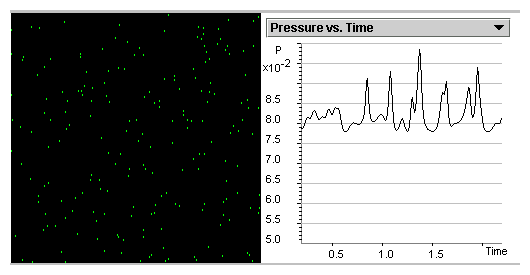
    2. Select Show Averages. Press Start. Watch the Pressure vs. Time graph for approximately 5.0 time units.

    You can see that the fluctuations of pressure are rather significant and the values on the Average Values panel are constantly changing. In order to obtain accurate measurements, you need to average data for significantly longer times, such as 20 time units.


    3. Change Iterations Between Displays to 500. Let the program run for approximately 20 computer time units as shown in figure 2.4. Press Pause.

    Setting Iterations Between Displays at 500 speeds up the simulation.

figures2/pic4c.png

Figure 2.4: Screenshot of Gay-Lussac's Law SimuLab.


    4. Record the pressure from the Average Values panel for this trial in your Table for T=4. Calculate the  P/T value. Press Reset Averages on the Average Values panel.

    You are preparing data for the future analysis.


    5. Set the Temperature to T=3. Press Start. Let the program run for 20 time units. Press Pause. Record Pressure and calculate P/T ratio. Select Reset Averages on the Average Values panel.
      Ressetting Averages allows you to delete the data values from the previous experiment.


    6. Repeat Step 5 for Temperatures T=2, T=1.25,and T=1.


Q2.41: Compare the values of P/T obtained for various temperatures with the average value of P/T from the table. | (  P/T)i - (  P/T )avg |. Express the differences in percents


ê
ê
æ
è
 P

T
ö
ø
i 
- æ
è
 P

T
ö
ø
avg 
ê
ê

æ
è
 P

T
ö
ø
avg 
×100


and record them into the table.


Q2.42: What conclusions can you draw about the consistency of the  P/T constant in relation to temperature?


Q2.43: Plot a Pressure vs. Temperature graph. Approximate it by a straight line. Determine the slope of the graph. Extrapolate the line to P=0.


Q2.44: What is the temperature when P=0? Explain your result.